Quantifying uncertainty

Lecture 24

Author

Affiliation

Dr. Mine Çetinkaya-Rundel

Duke University
STA 199 - Fall 2025

Warm-up

While you wait: Participate 📱💻

Given that HW 6 will be assigned on Monday, Dec 1, what day should HW 5 be due? It will be due at 11:59 pm on the deadline we decide on.

• Sunday, Nov 30 - no change
• Monday, Dec 1 - postponed by 1 day
• Tuesday, Dec 2 - postponed by 2 days
• Wednesday, Dec 3 - postponed by 3 days

Scan the QR code or go to app.wooclap.com/sta199. Log in with your Duke NetID.

Announcements

• HW:
  • HW 5 due [whichever date we decided on in the previous slide]
  • HW 6 due at 11:59 pm on Fri, Dec 6, but will be accepted until Sun, Dec 7 at 11:59 pm without penalty
• Final exam:
  • In-class only, “cheat sheet” with same specs as usual allowed
  • Cumulative – will definitely have material since Exam 2, but there’s so little of it that it won’t be a huge portion of the exam
  • Final exam review during reading period – date/time/location TBA
  • Office hours during reading period + final exam week – schedule TBA
• Grades:
  • Exam 2 in-class grades posted – can review questions in my office hours anytime before the final
  • Exam 2 take-home + project grades to be posted after Thanksgiving break

Quantifying uncertainty

Goal

Find range of plausible values for the slope using bootstrap confidence intervals.

Packages

# load packages
library(tidyverse) # for data wrangling and visualization
library(tidymodels) # for modeling
library(openintro) # for Duke Forest dataset
library(scales) # for pretty axis labels
library(glue) # for constructing character strings
library(knitr) # for neatly formatted tables

Data: Houses in Duke Forest

• Data on houses that were sold in the Duke Forest neighborhood of Durham, NC around November 2020
• Scraped from Zillow
• Source: openintro::duke_forest

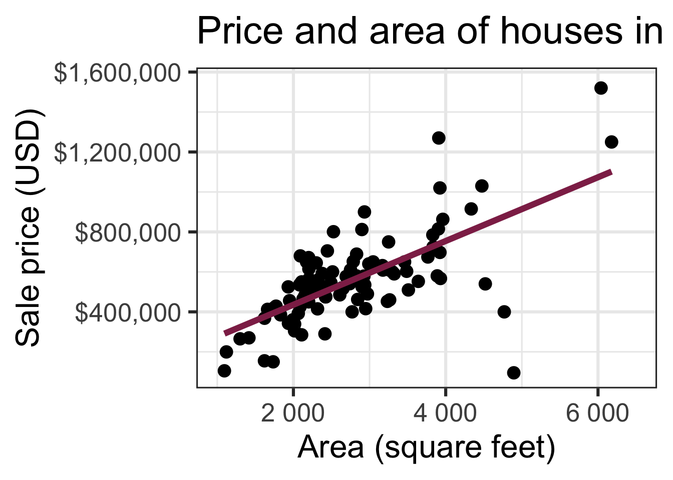
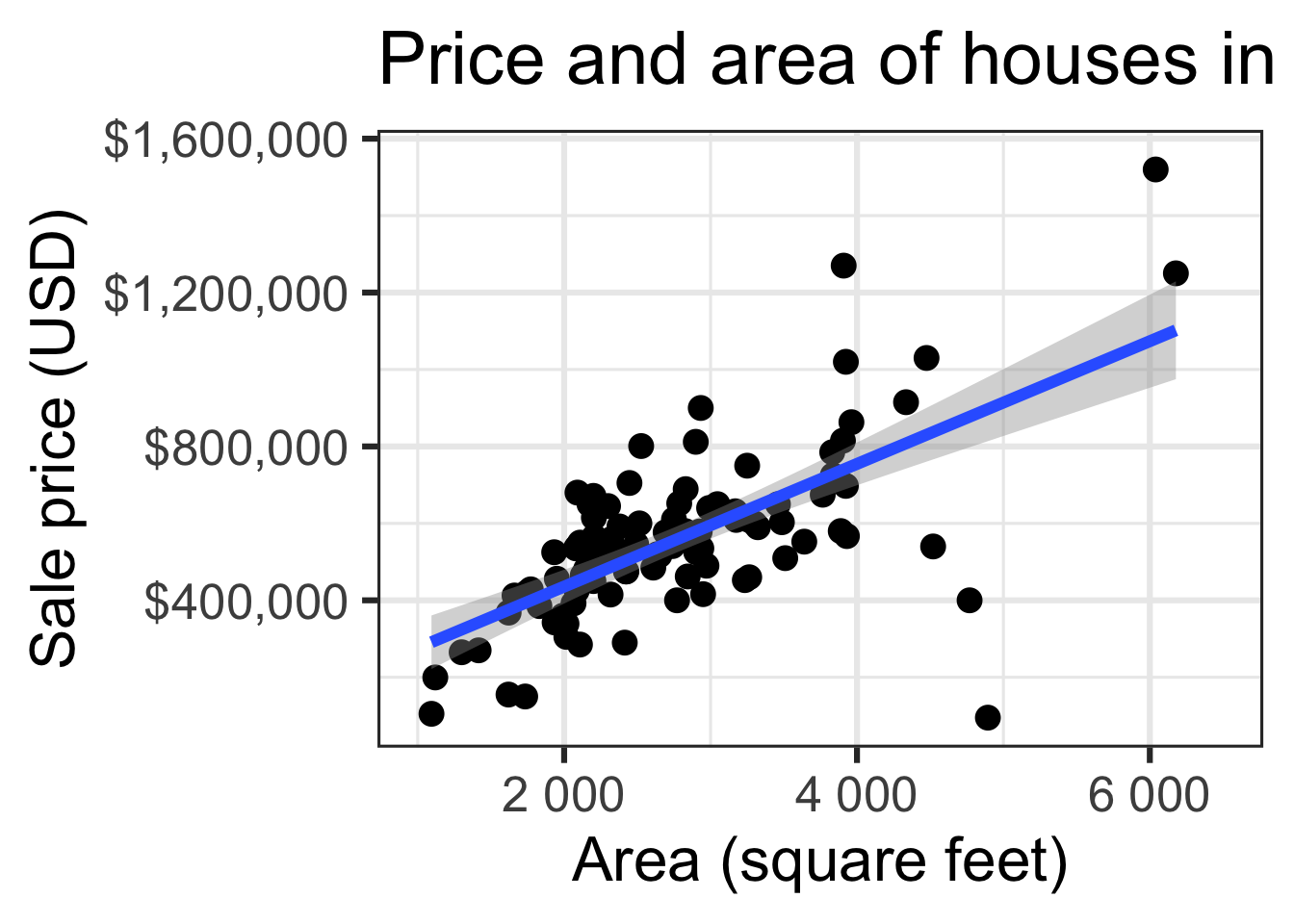
Goal: Use the area (in square feet) to understand variability in the price of houses in Duke Forest.

Exploratory data analysis

ggplot(duke_forest, aes(x = area, y = price)) +
  geom_point(alpha = 0.7) +
  labs(
    x = "Area (square feet)",
    y = "Sale price (USD)",
    title = "Price and area of houses in Duke Forest"
  ) +
  scale_y_continuous(labels = label_dollar())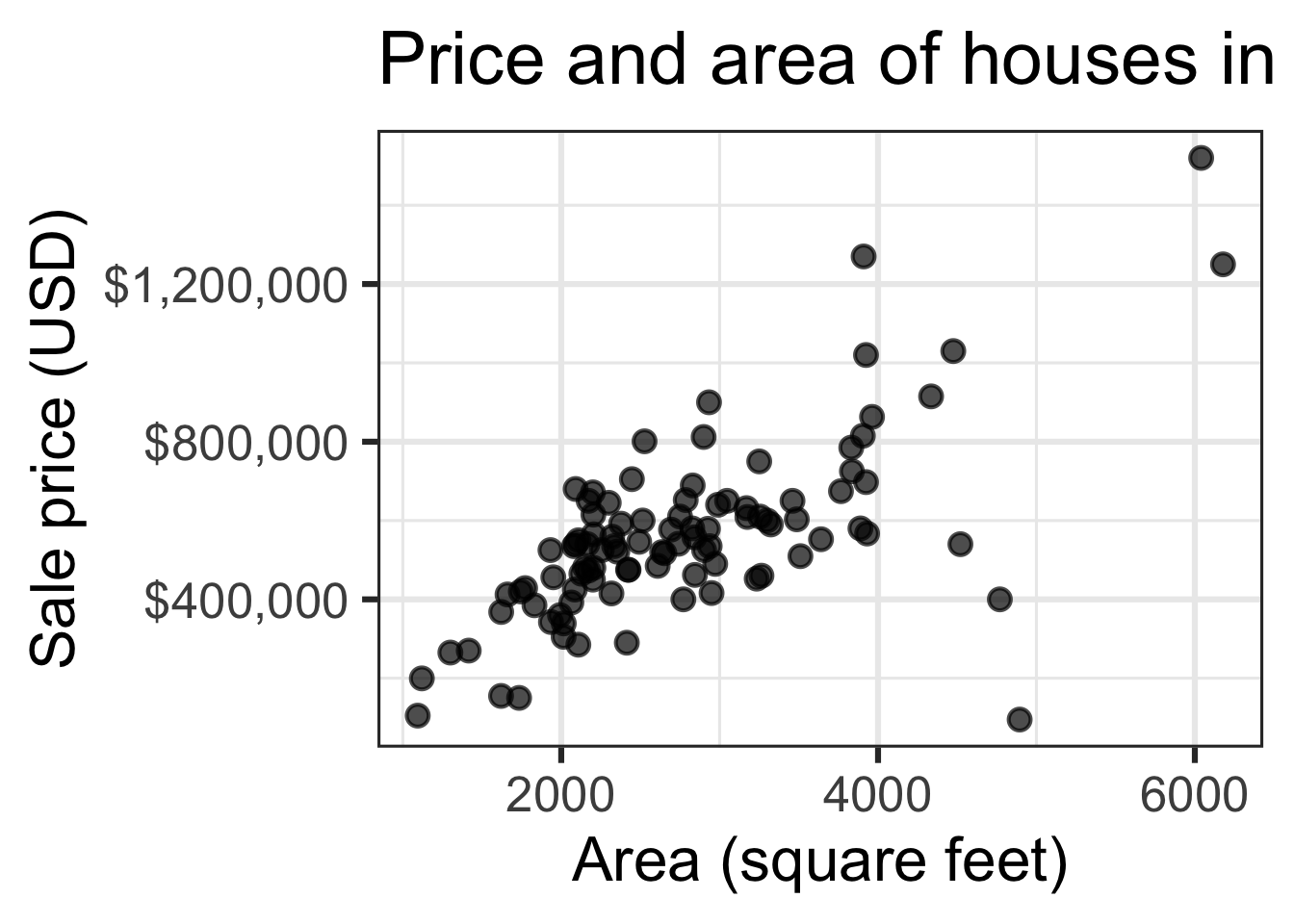

Modeling

df_fit <- linear_reg() |>
  fit(price ~ area, data = duke_forest)

tidy(df_fit) |>
  kable(digits = 2) # neatly format table to 2 digits

term	estimate	std.error	statistic	p.value
(Intercept)	116652.33	53302.46	2.19	0.03
area	159.48	18.17	8.78	0.00

Participate 📱💻

Which of the following is the correct interpretation of the intercept?

term	estimate	std.error	statistic	p.value
(Intercept)	116652	53302	2	0
area	159	18	9	0

• For each additional square foot, the model predicts the sale price of Duke Forest houses to be higher by $116,652, on average.
• Duke Forest houses that are 0 square feet are predicted to sell, for $116,652, on average.
• For each additional square foot, the model predicts the sale price of Duke Forest houses to be lower by $15,900, on average.
• Duke Forest houses that are 0 square feet are predicted to sell, for $15,900, on average.

Scan the QR code or go to app.wooclap.com/sta199. Log in with your Duke NetID.

Participate 📱💻

Which of the following is the correct interpretation of the slope?

term	estimate	std.error	statistic	p.value
(Intercept)	116652	53302	2	0
area	159	18	9	0

• For each additional square foot, the model predicts the sale price of Duke Forest houses to be higher by $159, on average.
• Duke Forest houses that are 0 square feet are predicted to sell, for $116,652, on average.
• For each additional square foot, the model predicts the sale price of Duke Forest houses to be lower by $15,900, on average.
• Duke Forest houses that are 0 square feet are predicted to sell, for $159, on average.

Scan the QR code or go to app.wooclap.com/sta199. Log in with your Duke NetID.

From sample to population

For each additional square foot, we expect the sale price of Duke Forest houses to be higher by $159, on average.

• This estimate is valid for the single sample of 98 houses.
• But what if we’re not interested quantifying the relationship between the size and price of a house in this single sample?
• What if we want to say something about the relationship between these variables for all houses in Duke Forest?

Statistical inference

• Statistical inference provide methods and tools so we can use the single observed sample to make valid statements (inferences) about the population it comes from

• For our inferences to be valid, the sample should be random and representative of the population we’re interested in

Inference for simple linear regression

• Calculate a confidence interval for the slope, \(\beta_1\) (today)

• Conduct a hypothesis test for the slope,\(\beta_1\) (next week)

Confidence interval for the slope

Confidence interval

• A plausible range of values for a population parameter is called a confidence interval
• Using only a single point estimate is like fishing in a murky lake with a spear, and using a confidence interval is like fishing with a net
  • We can throw a spear where we saw a fish but we will probably miss, if we toss a net in that area, we have a good chance of catching the fish
  • Similarly, if we report a point estimate, we probably will not hit the exact population parameter, but if we report a range of plausible values we have a good shot at capturing the parameter

Confidence interval for the slope

A confidence interval will allow us to make a statement like “For each additional square foot, the model predicts the sale price of Duke Forest houses to be higher, on average, by $159, plus or minus X dollars.”

. . .

• Should X be $10? $100? $1000?

• If we were to take another sample of 98 would we expect the slope calculated based on that sample to be exactly $159? Off by $10? $100? $1000?

• The answer depends on how variable (from one sample to another sample) the sample statistic (the slope) is

• We need a way to quantify the variability of the sample statistic

Quantify the variability of the slope

for estimation

• Two approaches:
  1. Via simulation (what we’ll do in this course)
  2. Via mathematical models (what you can learn about in future courses)
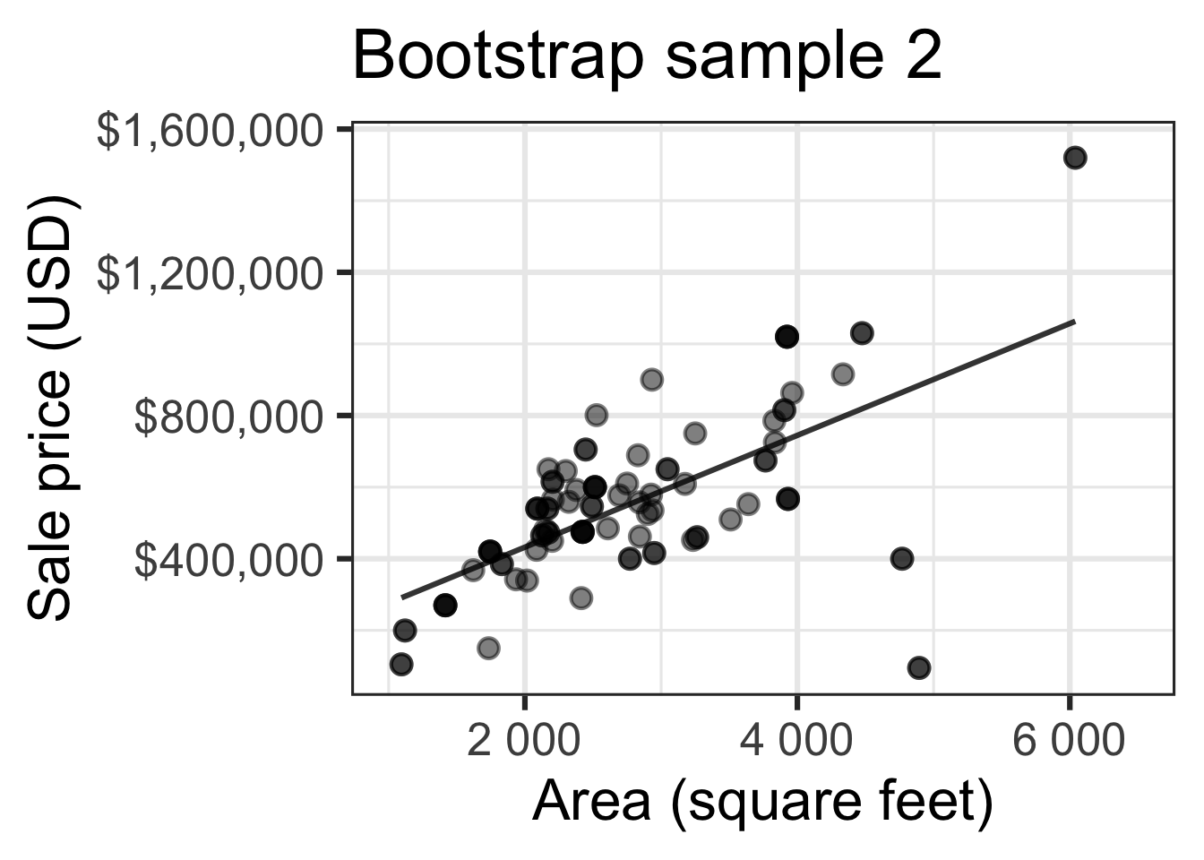
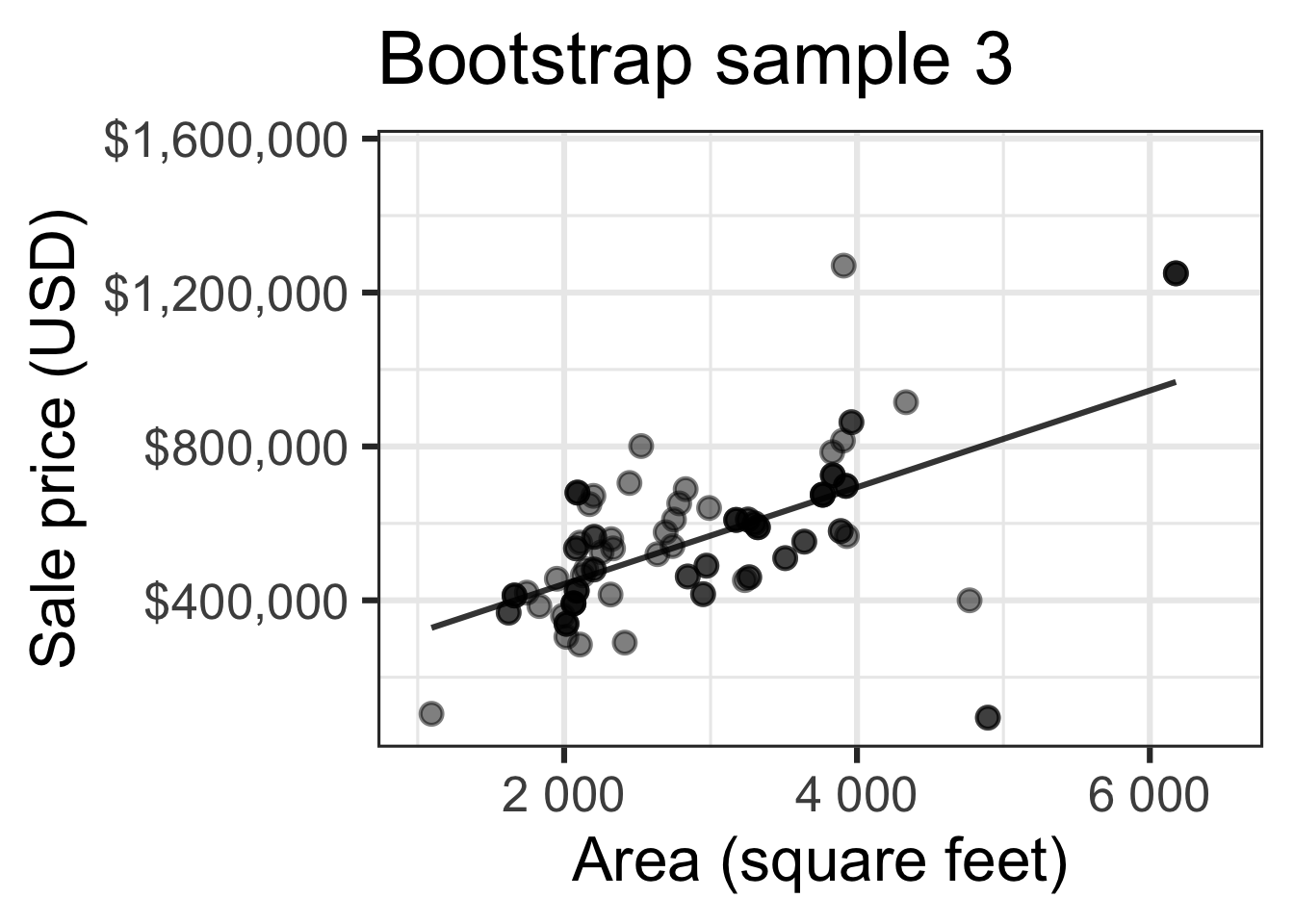
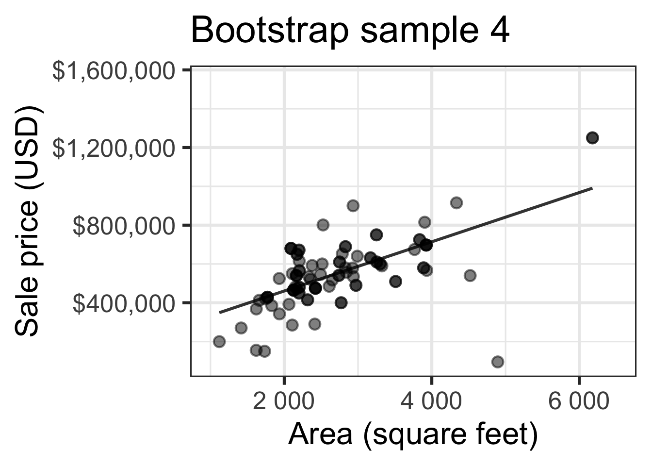
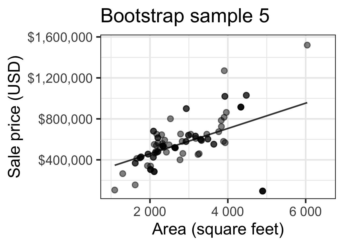
• Bootstrapping to quantify the variability of the slope for the purpose of estimation:
  • Bootstrap new samples from the original sample
  • Fit models to each of the samples and estimate the slope
  • Use features of the distribution of the bootstrapped slopes to construct a confidence interval

Bootstrap sample 1

Bootstrap sample 2

Bootstrap sample 3

Bootstrap sample 4

Bootstrap sample 5

. . .

so on and so forth…

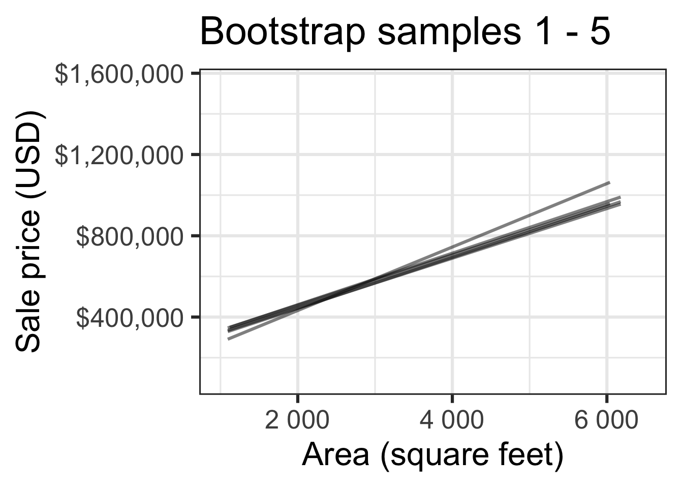
Bootstrap samples 1 - 5

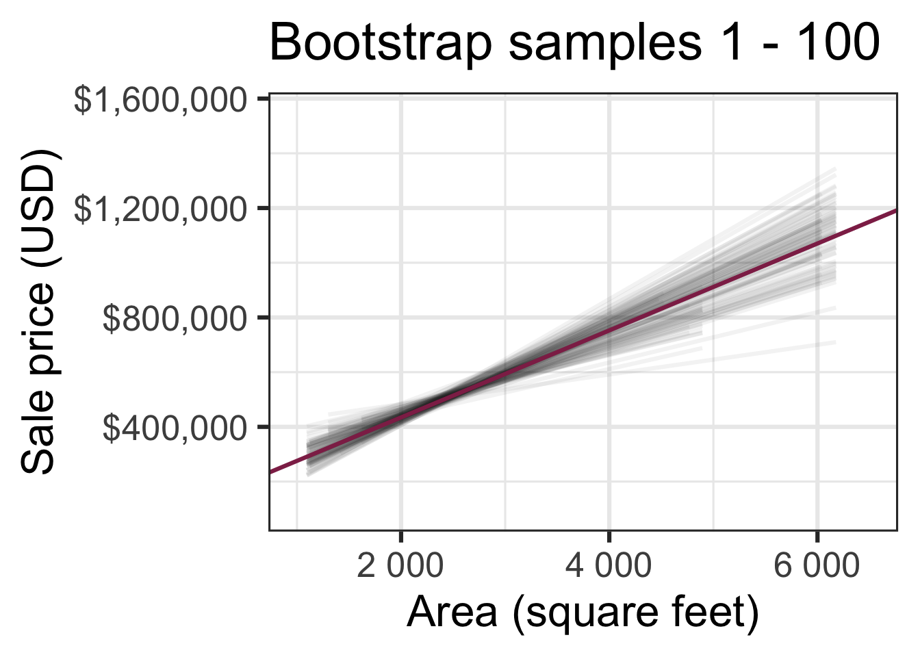
Bootstrap samples 1 - 100

. . .

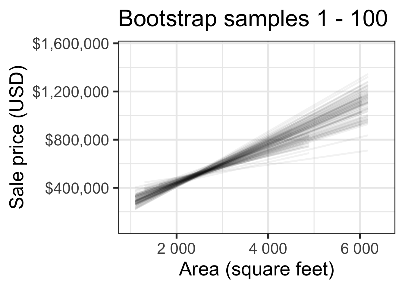
Look familiar?

Look familiar?

Slopes of bootstrap samples

Fill in the blank: For each additional square foot, the model predicts the sale price of Duke Forest houses to be higher, on average, by $159, plus or minus ___ dollars.

Slopes of bootstrap samples

Fill in the blank: For each additional square foot, we expect the sale price of Duke Forest houses to be higher, on average, by $159, plus or minus ___ dollars.

Confidence level

How confident are you that the true slope is between $0 and $250? How about $150 and $170? How about $90 and $210?

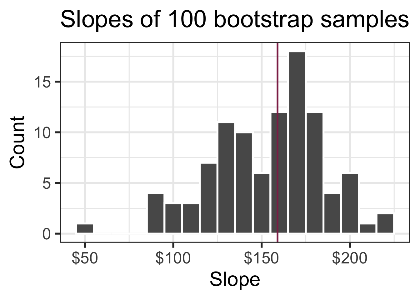
95% confidence interval

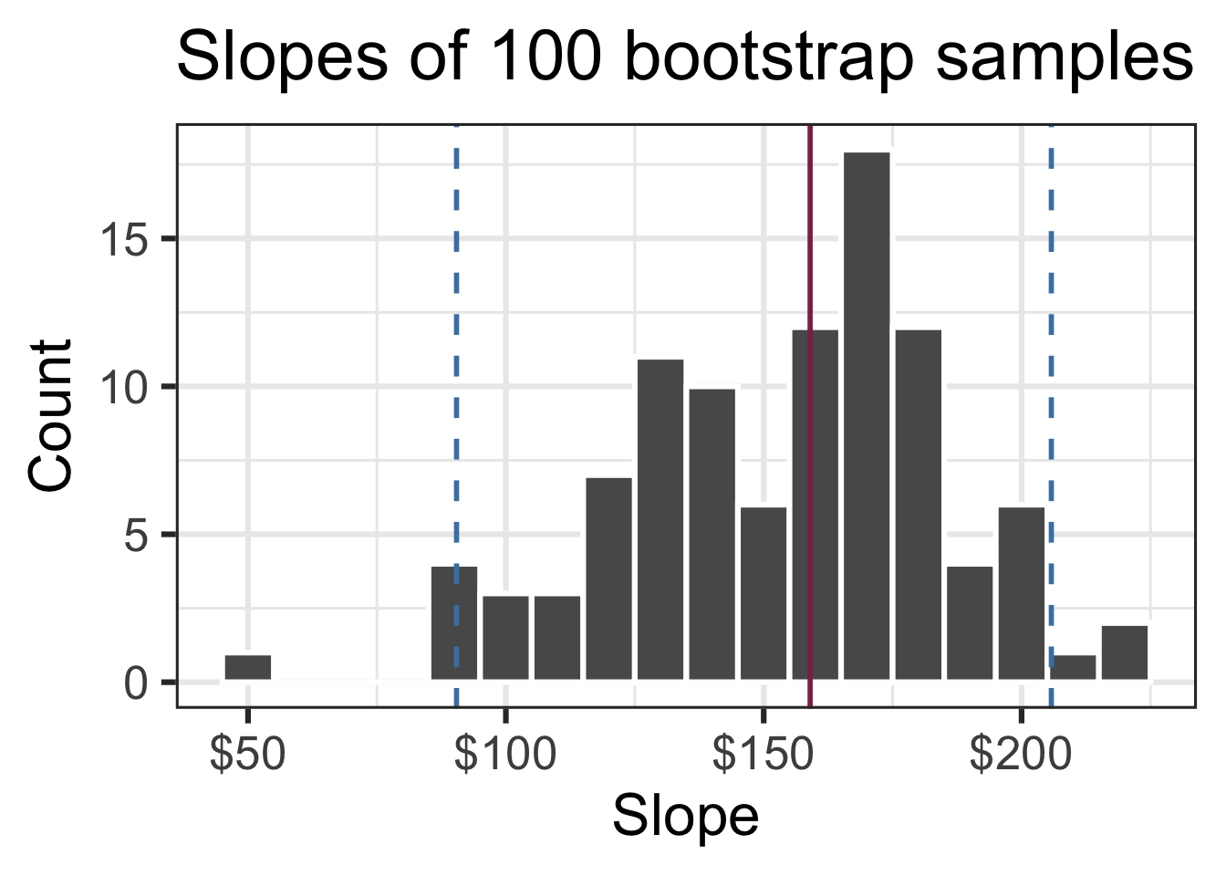
• A 95% confidence interval is bounded by the middle 95% of the bootstrap distribution
• We are 95% confident that for each additional square foot, the model predicts the sale price of Duke Forest houses to be higher, on average, by $90.43 to $205.77.

Application exercise

ae-15-duke-forest-bootstrap

• Go to your ae project in RStudio.

• If you haven’t yet done so, make sure all of your changes up to this point are committed and pushed, i.e., there’s nothing left in your Git pane.

• If you haven’t yet done so, click Pull to get today’s application exercise file: ae-15-duke-forest-bootstrap.qmd.

• Work through the application exercise in class, and render, commit, and push your edits.