Quantifying uncertainty
Lecture 24
November 25, 2025
While you wait: Participate 📱💻
Given that HW 6 will be assigned on Monday, Dec 1, what day should HW 5 be due? It will be due at 11:59 pm on the deadline we decide on.
- Sunday, Nov 30 - no change
- Monday, Dec 1 - postponed by 1 day
- Tuesday, Dec 2 - postponed by 2 days
- Wednesday, Dec 3 - postponed by 3 days

Scan the QR code or go to app.wooclap.com/sta199. Log in with your Duke NetID.
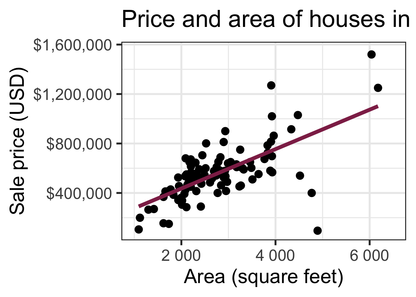
Data: Houses in Duke Forest
- Data on houses that were sold in the Duke Forest neighborhood of Durham, NC around November 2020
- Scraped from Zillow
- Source:
openintro::duke_forest
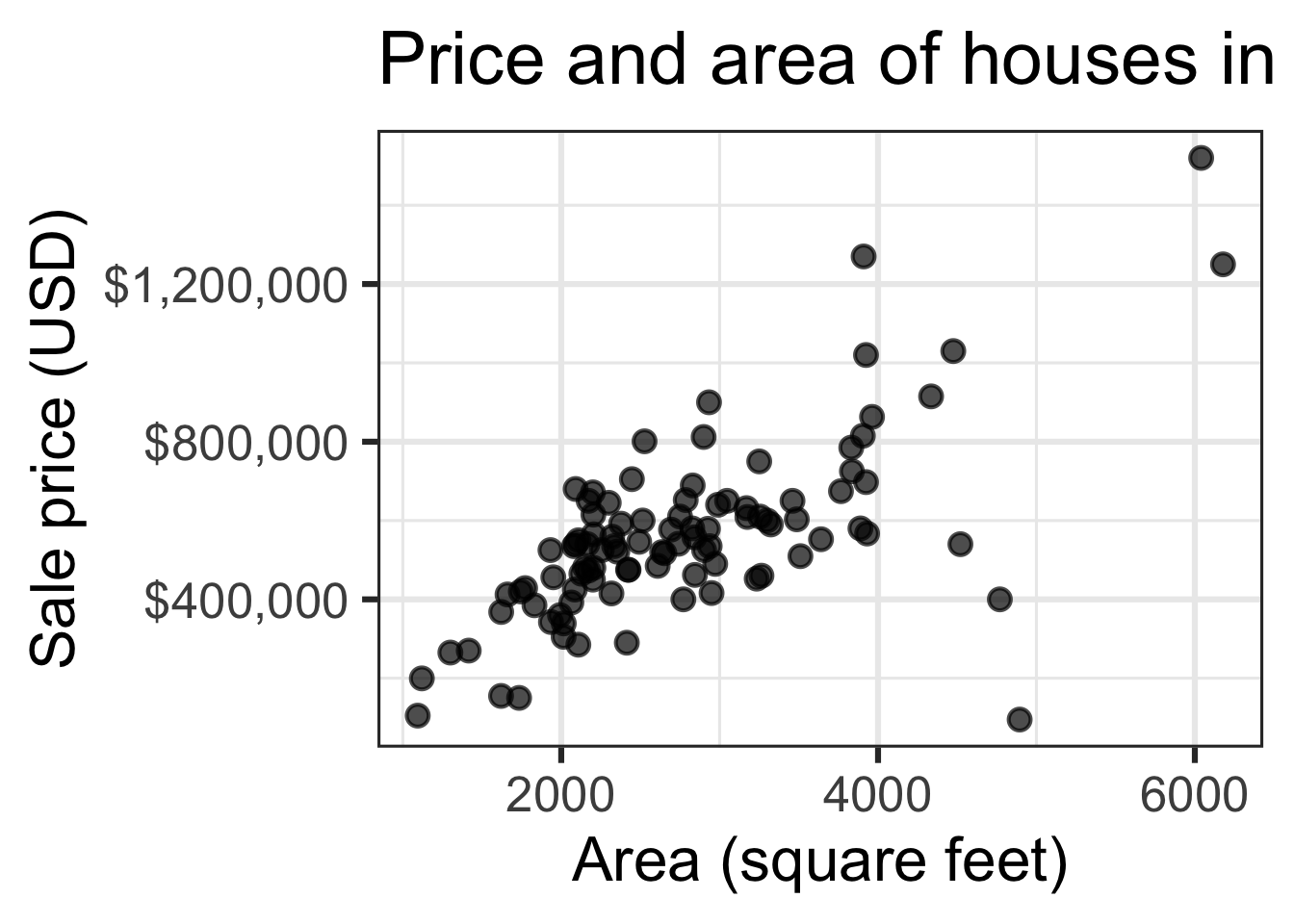
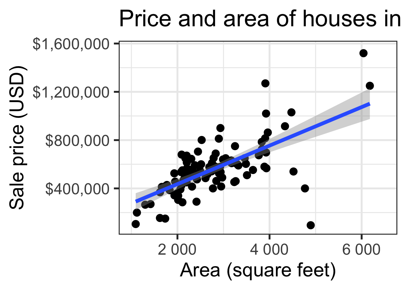
Goal: Use the area (in square feet) to understand variability in the price of houses in Duke Forest.
Exploratory data analysis
Participate 📱💻
Which of the following is the correct interpretation of the intercept?
| term | estimate | std.error | statistic | p.value |
|---|---|---|---|---|
| (Intercept) | 116652 | 53302 | 2 | 0 |
| area | 159 | 18 | 9 | 0 |
- For each additional square foot, the model predicts the sale price of Duke Forest houses to be higher by $116,652, on average.
- Duke Forest houses that are 0 square feet are predicted to sell, for $116,652, on average.
- For each additional square foot, the model predicts the sale price of Duke Forest houses to be lower by $15,900, on average.
- Duke Forest houses that are 0 square feet are predicted to sell, for $15,900, on average.
Scan the QR code or go to app.wooclap.com/sta199. Log in with your Duke NetID.
Participate 📱💻
Which of the following is the correct interpretation of the slope?
| term | estimate | std.error | statistic | p.value |
|---|---|---|---|---|
| (Intercept) | 116652 | 53302 | 2 | 0 |
| area | 159 | 18 | 9 | 0 |
- For each additional square foot, the model predicts the sale price of Duke Forest houses to be higher by $159, on average.
- Duke Forest houses that are 0 square feet are predicted to sell, for $116,652, on average.
- For each additional square foot, the model predicts the sale price of Duke Forest houses to be lower by $15,900, on average.
- Duke Forest houses that are 0 square feet are predicted to sell, for $159, on average.
Scan the QR code or go to app.wooclap.com/sta199. Log in with your Duke NetID.
Statistical inference
Statistical inference provide methods and tools so we can use the single observed sample to make valid statements (inferences) about the population it comes from
For our inferences to be valid, the sample should be random and representative of the population we’re interested in

Bootstrap sample 1


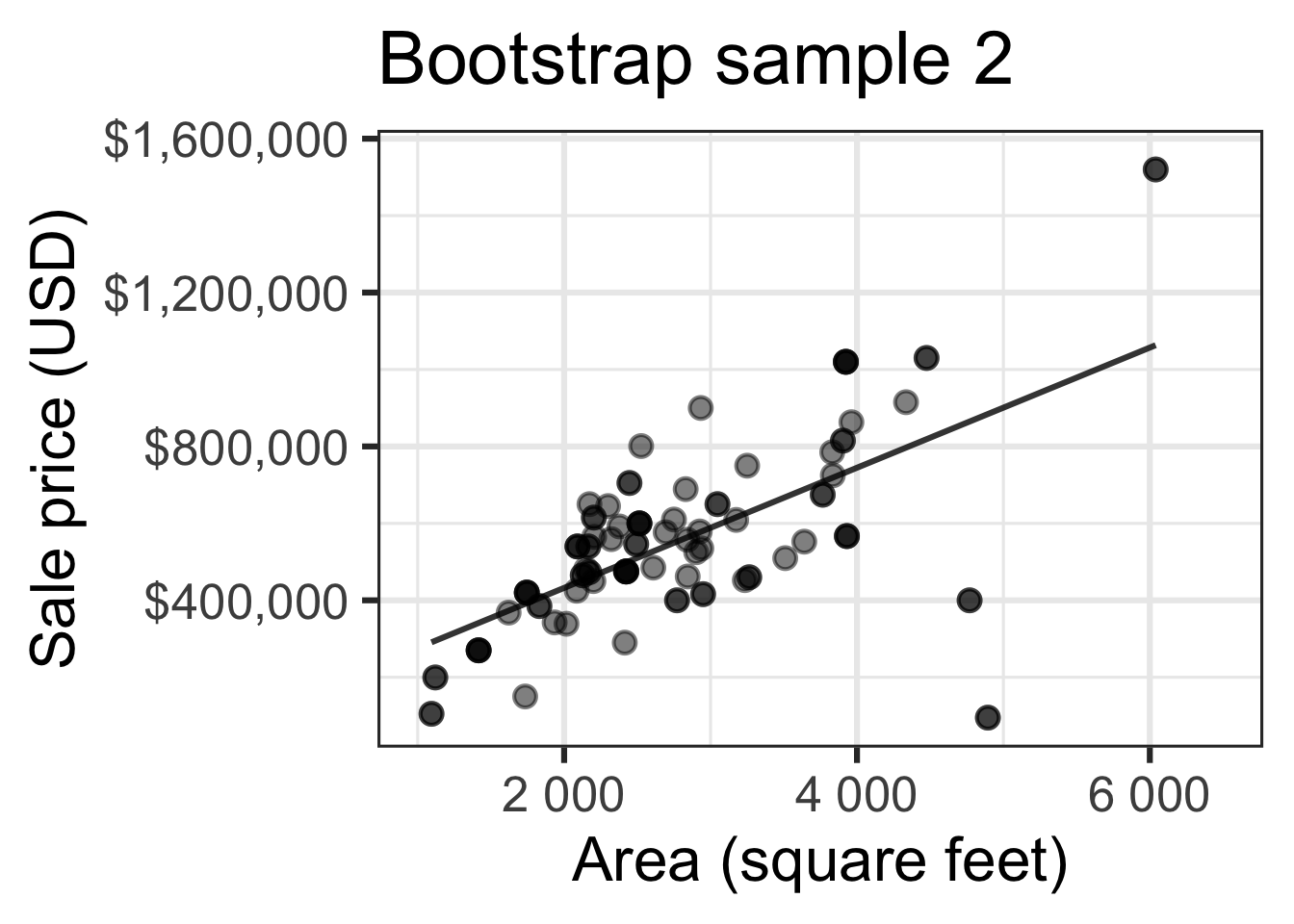
Bootstrap sample 2

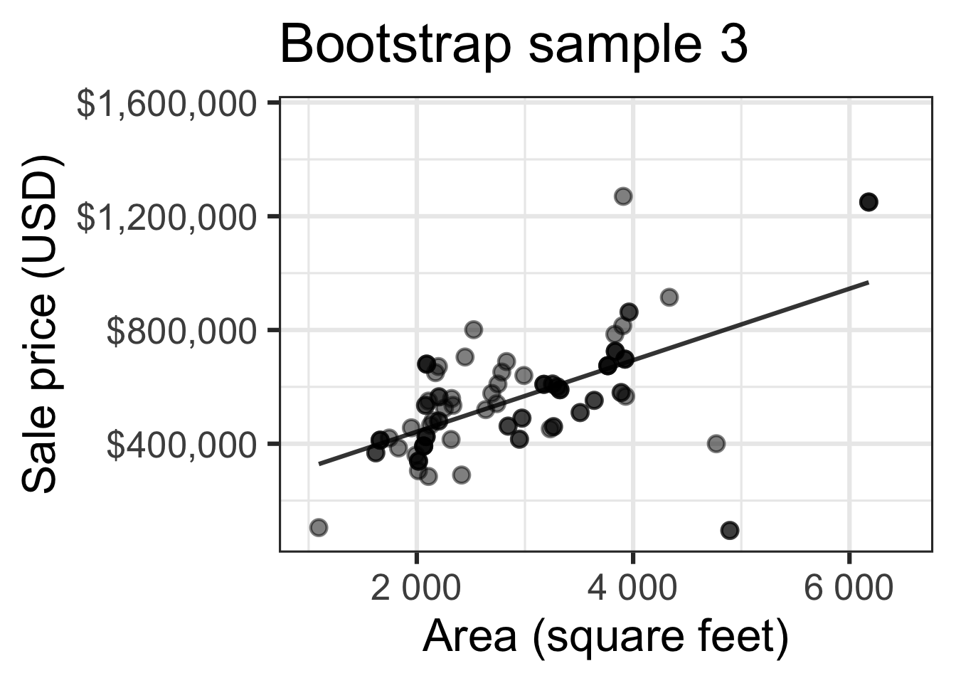
Bootstrap sample 3

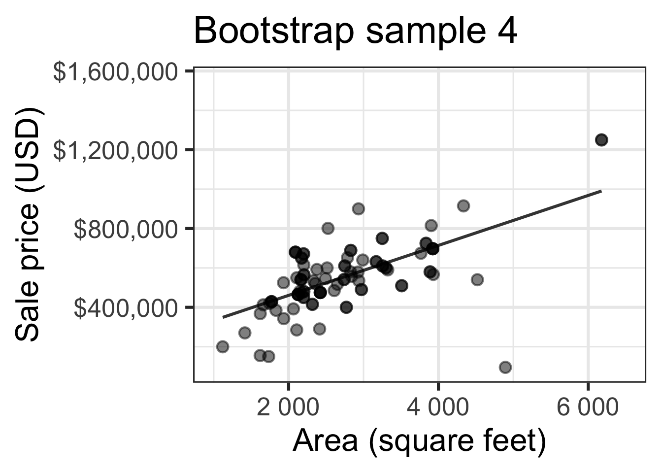
Bootstrap sample 4
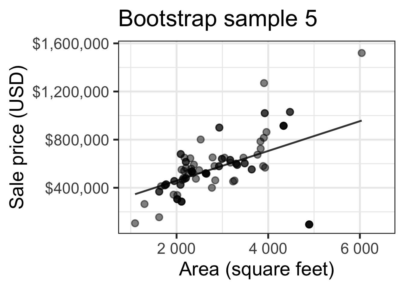
Bootstrap sample 5

so on and so forth…
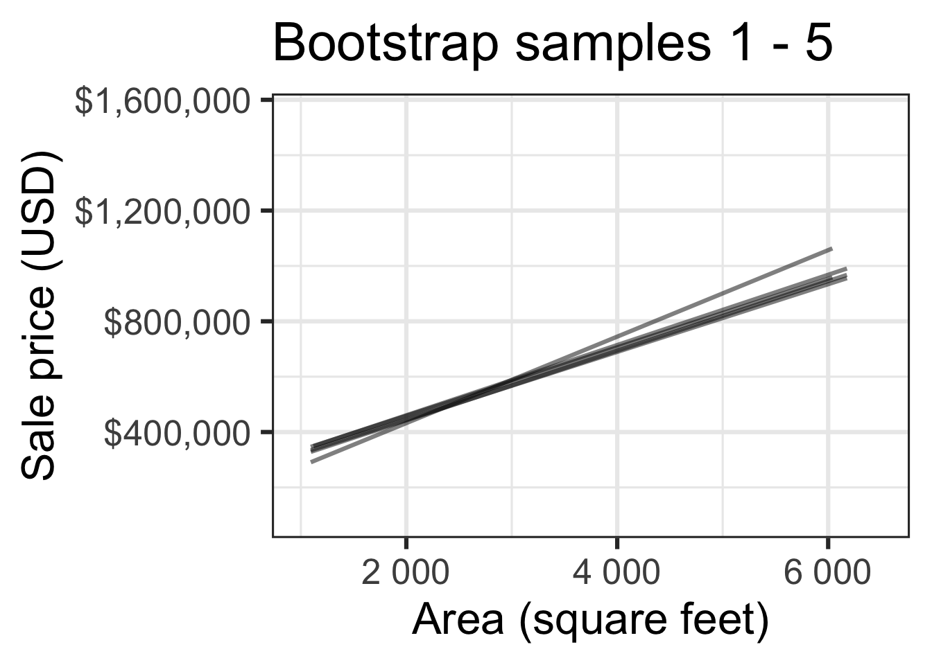
Bootstrap samples 1 - 5

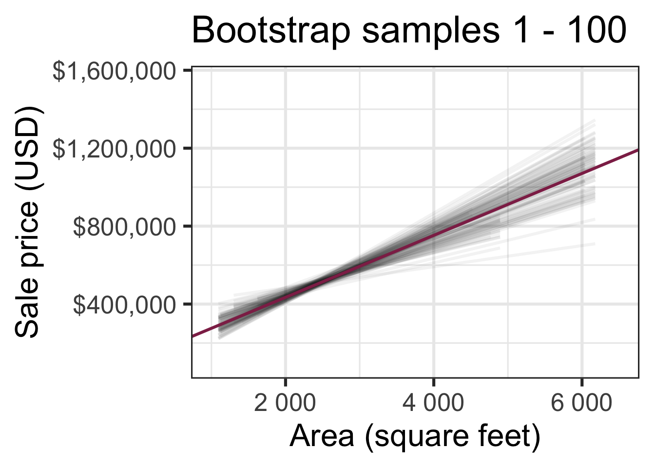
Bootstrap samples 1 - 100

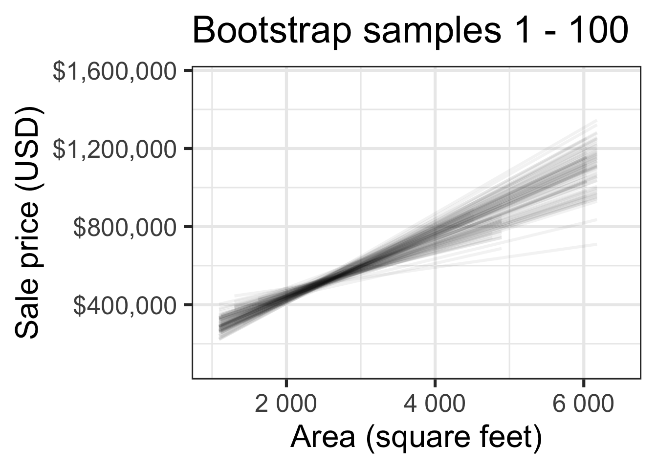
Look familiar?
Look familiar?

Slopes of bootstrap samples
Fill in the blank: For each additional square foot, the model predicts the sale price of Duke Forest houses to be higher, on average, by $159, plus or minus ___ dollars.
Slopes of bootstrap samples
Fill in the blank: For each additional square foot, we expect the sale price of Duke Forest houses to be higher, on average, by $159, plus or minus ___ dollars.

Confidence level
How confident are you that the true slope is between $0 and $250? How about $150 and $170? How about $90 and $210?
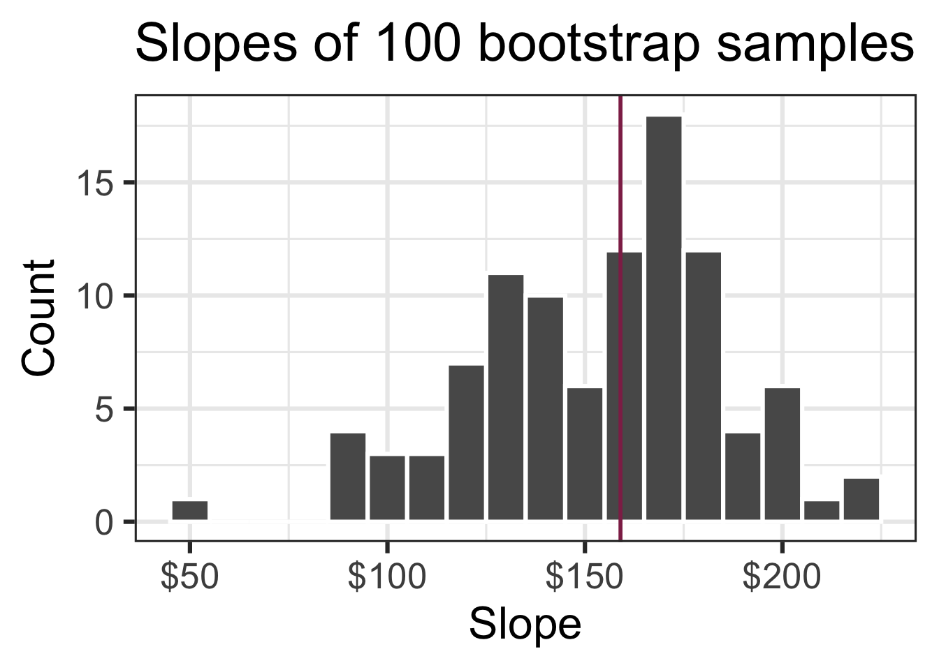
95% confidence interval
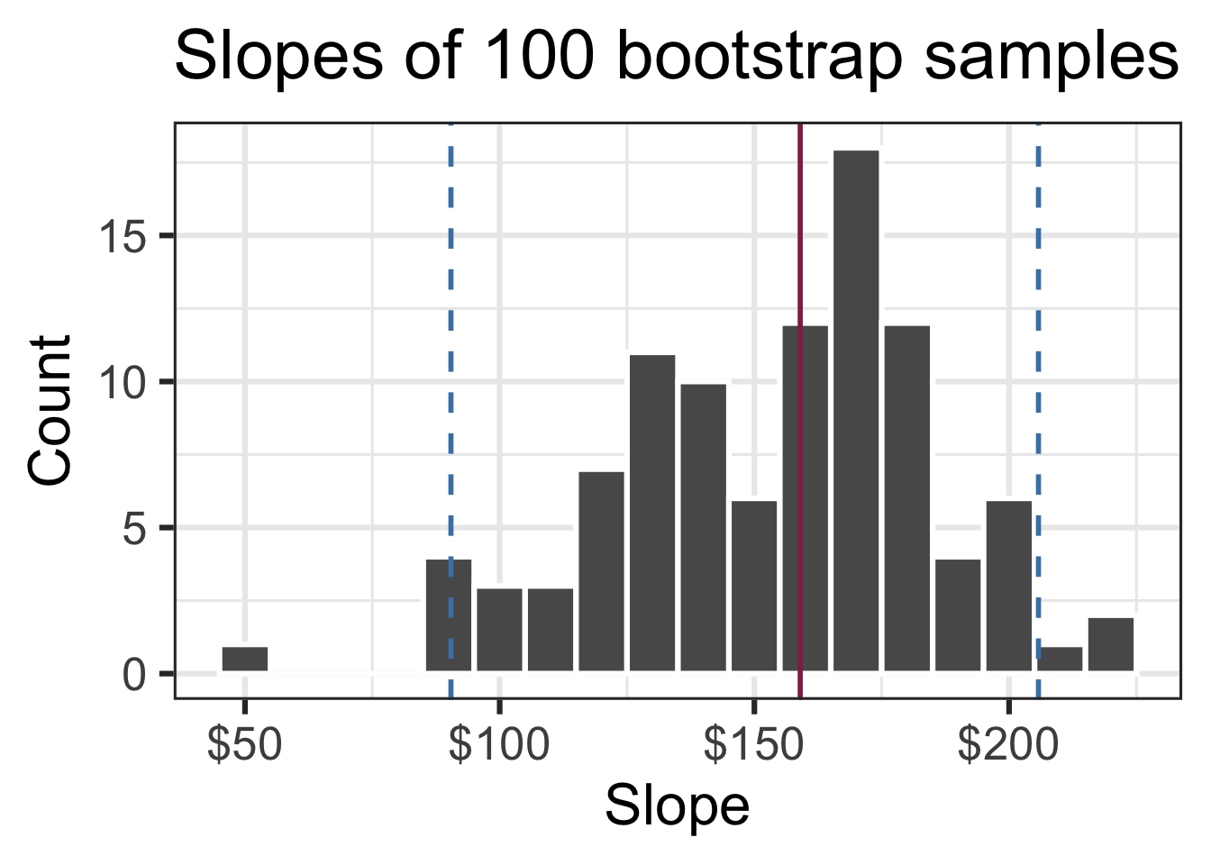
- A 95% confidence interval is bounded by the middle 95% of the bootstrap distribution
- We are 95% confident that for each additional square foot, the model predicts the sale price of Duke Forest houses to be higher, on average, by $90.43 to $205.77.