Logistic regression

Lecture 20

Author

Affiliation

Dr. Mine Çetinkaya-Rundel

Duke University
STA 199 - Fall 2025

Warm-up

Announcements

• My Friday office hours extended – 12:45 - 3:00 PM in for this week

• Project presentations: Hard stop at 5 minute mark! No limit on number of slides, but be mindful of how long it takes you to go through each.

Project questions

• Focus: Can expand focus after research question, sure!

• Citations: Don’t have to have them on slides and don’t need to say them out loud unless relevant to presentation, must include in writeup.

• Vairble names: It’s ok to have some long variable names, but if you’re using them a lot in your code, make sure code is easy to follow.

• Outliers: Evaluate if they’re genuinely influencing your model.

• Grading: Rubric is in the milestone 6.

• Categorical variables + summary stats: Correlation isn’t appropriate, report %s or make stacked bar plots.

• There is no single correct number of graphs, tables, etc.

• Review your website by clicking on the link from your repo.

• Analysis writeup can be broken into multiple pieces with plots, tables, etc. sprinkled.

• Who is grading? TAs and myself, I’ll be at (most of) the presentations.

• When is it due?

Logistic regression

Packages

library(tidyverse) # data wrangling and visualization
library(tidymodels) # modeling
library(openintro) # emails data
library(fivethirtyeight) # movies data
library(palmerpenguins) # penguins data
library(ggthemes) # accessible color palettes

Thus far…

We have been studying regression:

• What combinations of data types have we seen?

• What did the picture look like?

Recap: Simple linear regression

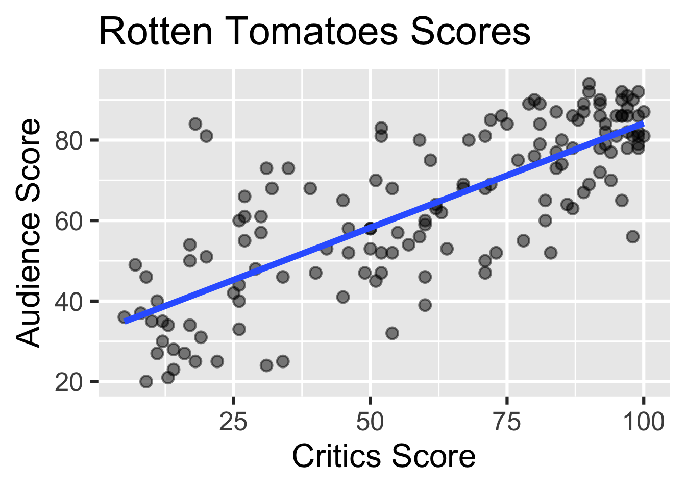
Numerical outcome and one numerical predictor:

Recap: Simple linear regression

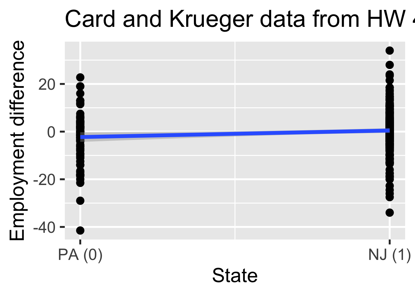
Numerical outcome and one categorical predictor (two levels):

Recap: Multiple linear regression

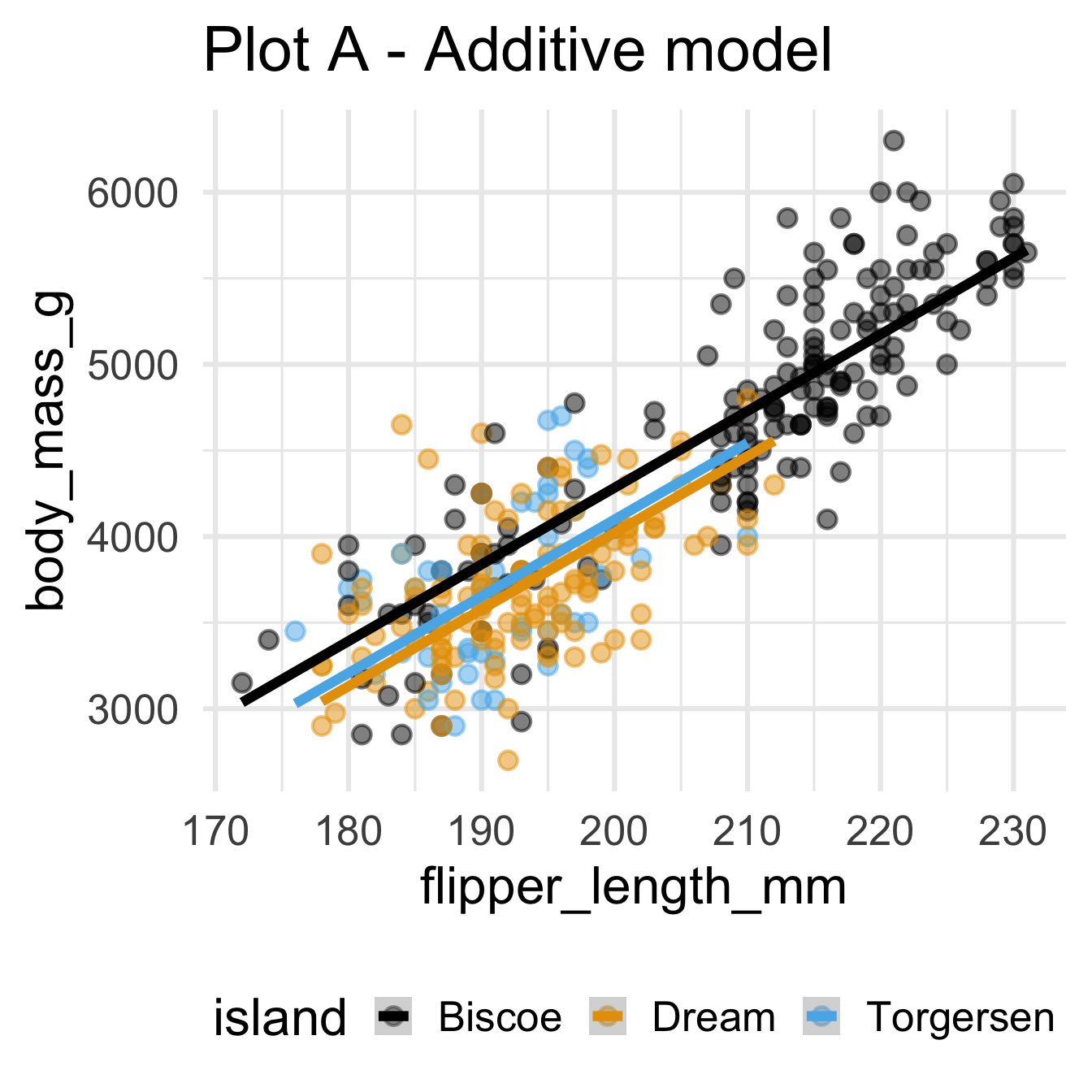
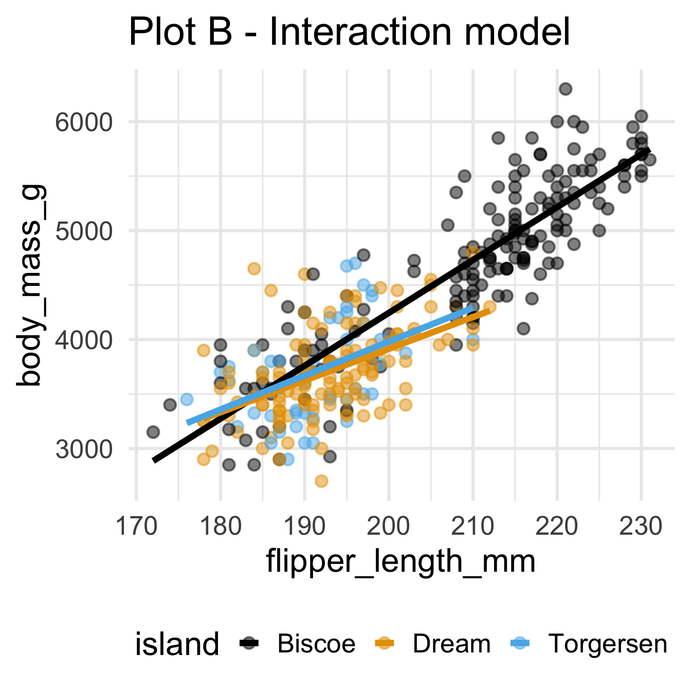
Numerical outcome, numerical and categorical predictors:

Today: a binary outcome

\[ y = \begin{cases} 1 & &&\text{eg. Yes, Win, True, Heads, Success}\\ 0 & &&\text{eg. No, Lose, False, Tails, Failure}. \end{cases} \]

Who cares?

If we can model the relationship between predictors (\(x\)) and a binary outcome (\(y\)), we can use the model to do a special kind of prediction called classification.

Example: Is the e-mail spam or not?

\[ \mathbf{x}: \text{word and character counts in an e-mail.} \]

\[ y = \begin{cases} 1 & \text{it's spam}\\ 0 & \text{it's legit} \end{cases} \]

Example: Is it cancer or not?

\[ \mathbf{x}: \text{features in a medical image.} \]

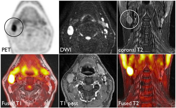
\[ y = \begin{cases} 1 & \text{it's cancer}\\ 0 & \text{it's healthy} \end{cases} \]

Example: Will they default?

\[ \mathbf{x}: \text{financial and demographic info about a loan applicant.} \]

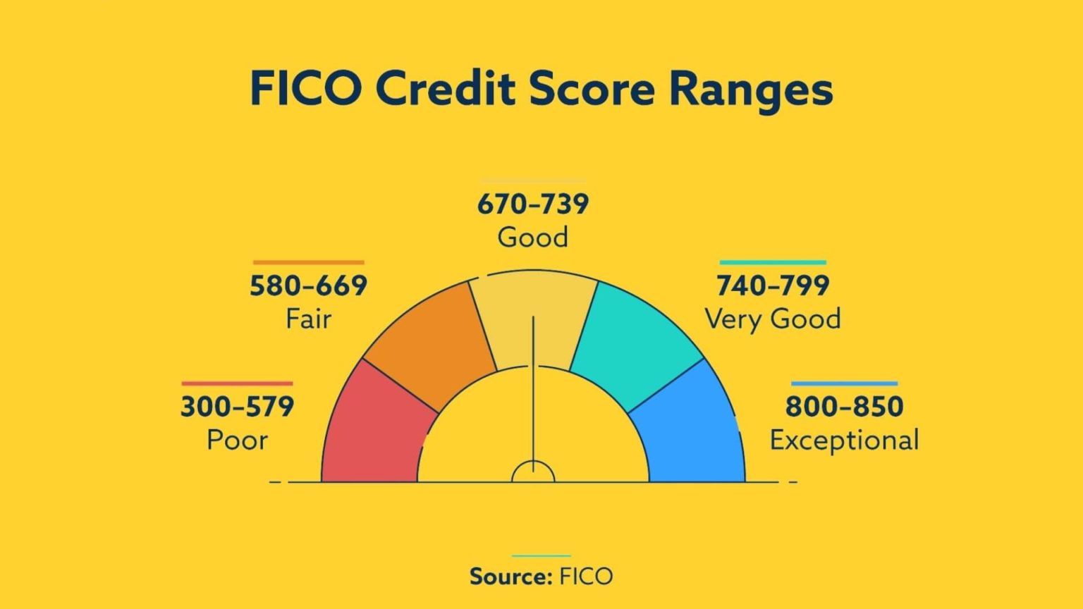
\[ y = \begin{cases} 1 & \text{applicant is at risk of defaulting on loan}\\ 0 & \text{applicant is safe} \end{cases} \]

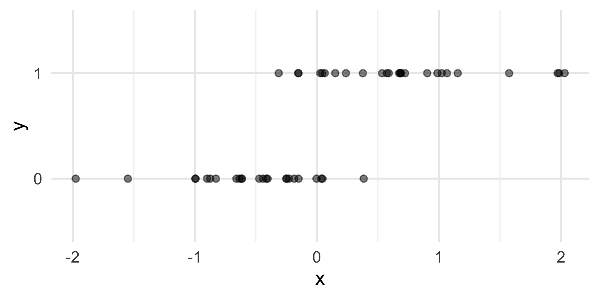
How do we model this type of data?

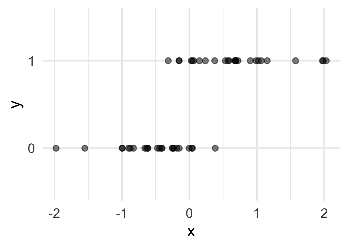
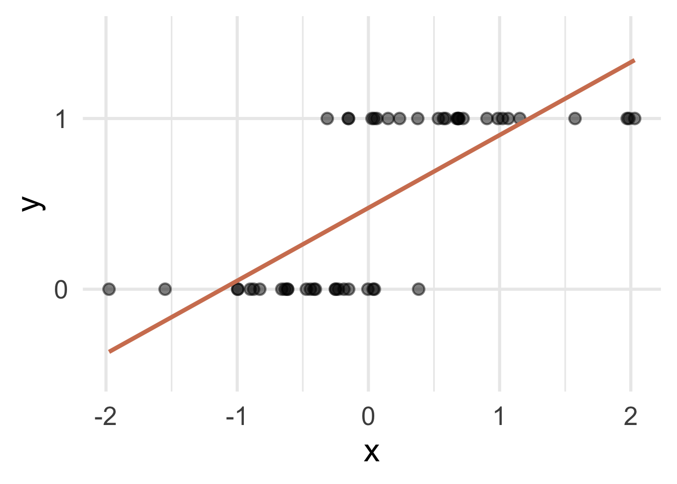
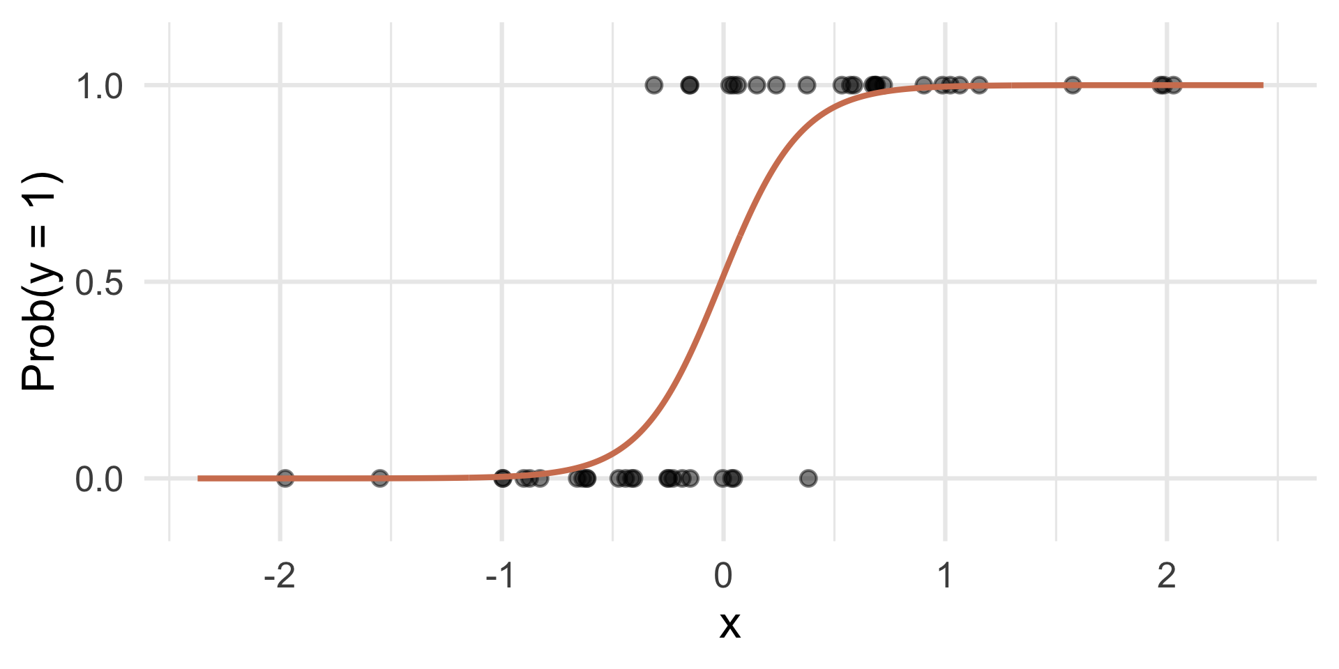
Straight line of best fit is a little silly

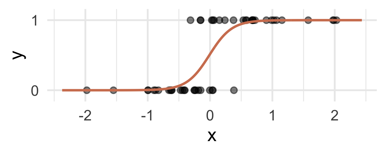
Instead: S-curve of best fit

Instead of modeling \(y\) directly, we model the probability that \(y=1\):

• “Given new email, what’s the probability that it’s spam?’’
• “Given new image, what’s the probability that it’s cancer?’’
• “Given new loan application, what’s the probability that they default?’’

Why don’t we model y directly?

• Recall regression with a numerical outcome:

  • Our models do not output guarantees for \(y\), they output predictions that describe behavior on average

• Similar when modeling a binary outcome:

  • Our models cannot directly guarantee that \(y\) will be zero or one. The correct analog to “on average” for a 0/1 outcome is “what’s the probability?”

So, what is this S-curve, anyway?

It’s the logistic function:

\[ \text{Prob}(y = 1) = \frac{e^{\beta_0+\beta_1x}}{1+e^{\beta_0+\beta_1x}}. \]

If you set \(p = \text{Prob}(y = 1)\) and do some algebra, you get the simple linear model for the log-odds:

\[ \log\left(\frac{p}{1-p}\right) = \beta_0+\beta_1x. \]

This is called the logistic regression model.

Log-odds?

• \(p = \text{Prob}(y = 1)\) is a probability. A number between 0 and 1

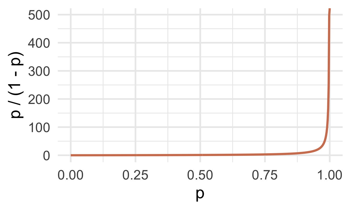
• \(p / (1 - p)\) is the odds. A number between 0 and \(\infty\)

“The odds of this lecture going well are 10 to 1.”

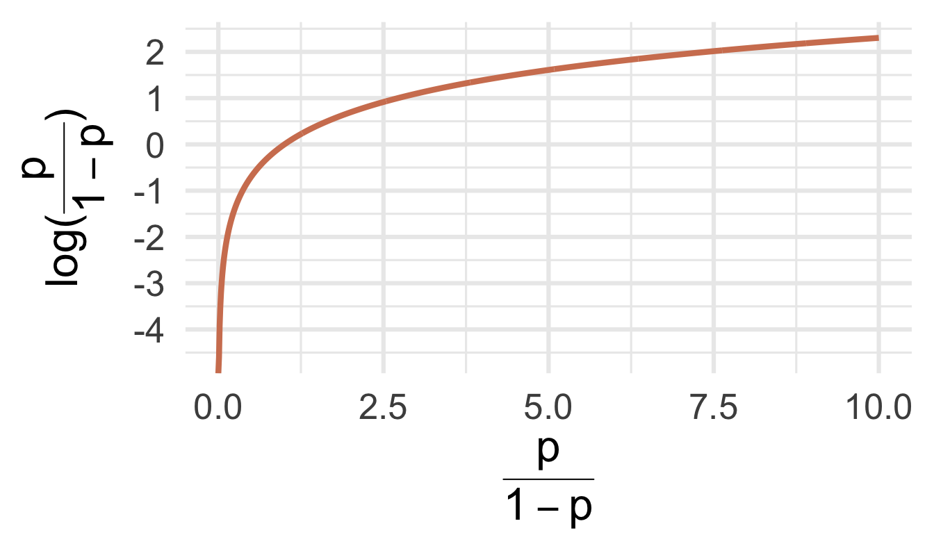
• The log odds \(\log(p / (1 - p))\) is a number between \(-\infty\) and \(\infty\), which is suitable for the linear model.

Probability to odds

Odds to log odds

Participate 📱💻

If \(p\) is the probability of success, what is the following called:

\[ \frac{p}{1-p} \]

• Probability of failure
• Odds of failure
• Odds of success
• Log-odds of success

Scan the QR code or go to app.wooclap.com/sta199. Log in with your Duke NetID.

Logistic regression

\[ \log\left(\frac{p}{1-p}\right) = \beta_0+\beta_1x. \]

• The logit function \(\log(p / (1-p))\) is an example of a link function that transforms the linear model to have an appropriate range

• This is an example of a generalized linear model

Estimation

• We estimate the parameters \(\beta_0\) (intercept) and \(\beta_1\) (slope) using maximum likelihood (don’t worry about it) to get the “best fitting” S-curve

• The fitted model is

\[ \log\left(\frac{\widehat{p}}{1-\widehat{p}}\right) = b_0+b_1x. \]

Today’s data

email |>
  select(c(spam, dollar, viagra, winner, password, exclaim_mess)) |>
  glimpse()

Rows: 3,921
Columns: 6
$ spam         <fct> 0, 0, 0, 0, 0, 0, 0, 0, 0, 0, 0, 0, 0, 0, 0, 0,…
$ dollar       <dbl> 0, 0, 4, 0, 0, 0, 0, 0, 0, 0, 0, 0, 0, 0, 2, 0,…
$ viagra       <dbl> 0, 0, 0, 0, 0, 0, 0, 0, 0, 0, 0, 0, 0, 0, 0, 0,…
$ winner       <fct> no, no, no, no, no, no, no, no, no, no, no, no,…
$ password     <dbl> 0, 0, 0, 0, 2, 2, 0, 0, 0, 0, 0, 0, 0, 0, 0, 0,…
$ exclaim_mess <dbl> 0, 1, 6, 48, 1, 1, 1, 18, 1, 0, 2, 1, 0, 10, 4,…

Fitting a logistic model

logistic_fit <- logistic_reg() |>
  fit(spam ~ exclaim_mess, data = email)

tidy(logistic_fit)

# A tibble: 2 × 5
  term          estimate std.error statistic p.value
  <chr>            <dbl>     <dbl>     <dbl>   <dbl>
1 (Intercept)  -2.27      0.0553     -41.1     0    
2 exclaim_mess  0.000272  0.000949     0.287   0.774

Fitted equation for the log-odds:

\[ \log\left(\frac{\hat{p}}{1-\hat{p}}\right) = -2.27 + 0.000272\times exclaim~mess \]

Interpreting the intercept

If exclaim_mess = 0, then

\[ \hat{p}=\widehat{P(y=1)}=\frac{e^{-2.27}}{1+e^{-2.27}}\approx 0.09. \]

So, an email with no exclamation marks has a 9% chance of being spam.

Interpreting the slope is tricky

Recall:

\[ \log\left(\frac{\widehat{p}}{1-\widehat{p}}\right) = b_0+b_1x. \]

. . .

Alternatively:

\[ \frac{\widehat{p}}{1-\widehat{p}} = e^{b_0+b_1x} = \color{blue}{e^{b_0}e^{b_1x}} . \]

. . .

If \(x\) is higher by one unit, we have:

\[ \frac{\widehat{p}}{1-\widehat{p}} = e^{b_0}e^{b_1(x+1)} = e^{b_0}e^{b_1x+b_1} = {\color{blue}{e^{b_0}e^{b_1x}}}{\color{red}{e^{b_1}}} . \]

. . .

A one unit increase in \(x\) is associated with a change in odds by a factor of \(e^{b_1}\). Helpful! 🙄

Back to the example…

\[ \log\left(\frac{\hat{p}}{1-\hat{p}}\right) = -2.27 + 0.000272\times exclaim~mess \]

Emails with one additional exclamation point are predicted to have odds of being spam that are higher by a factor of \(e^{0.000272}\approx 1.000272\), on average.

Classification
(logistic regression by another name…)

Step 1: fit the model

Select a number \(0 < p^* < 1\):

• if \(\text{Prob}(y=1)\leq p^*\), then predict \(\widehat{y}=0\)
• if \(\text{Prob}(y=1)> p^*\), then predict \(\widehat{y}=1\).

Step 2: pick a threshold

Select a number \(0 < p^* < 1\):

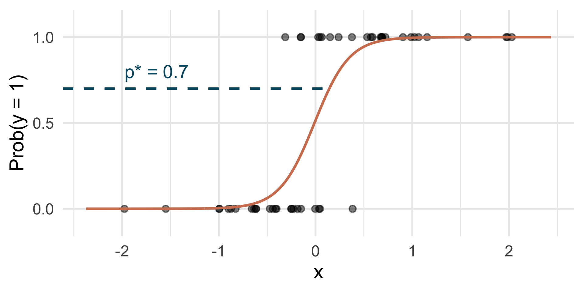
• if \(\text{Prob}(y=1)\leq p^*\), then predict \(\widehat{y}=0\)
• if \(\text{Prob}(y=1)> p^*\), then predict \(\widehat{y}=1\).

Step 3: find the “decision boundary”

Solve for the x-value that matches the threshold:

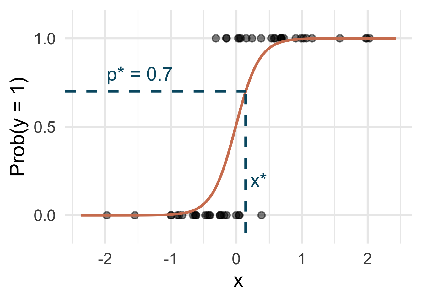
• if \(\text{Prob}(y=1)\leq p^*\), then predict \(\widehat{y}=0\)
• if \(\text{Prob}(y=1)> p^*\), then predict \(\widehat{y}=1\).

Step 4: classify a new arrival

A new person shows up with \(x_{\text{new}}\). Which side of the boundary are they on?

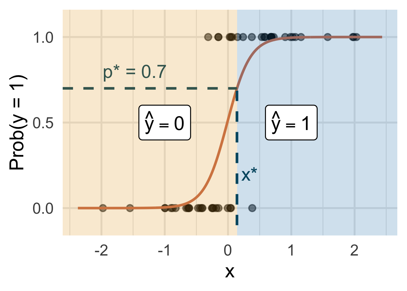
• if \(x_{\text{new}} \leq x^\star\), then \(\text{Prob}(y=1)\leq p^*\), so predict \(\widehat{y}=0\) for the new person
• if \(x_{\text{new}} > x^\star\), then \(\text{Prob}(y=1)> p^*\), so predict \(\widehat{y}=1\) for the new person.

Let’s change the threshold

A new person shows up with \(x_{\text{new}}\). Which side of the boundary are they on?

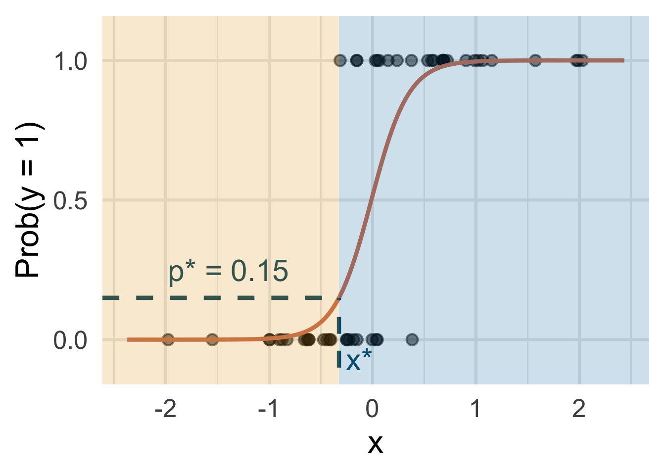
• if \(x_{\text{new}} \leq x^\star\), then \(\text{Prob}(y=1)\leq p^*\), so predict \(\widehat{y}=0\) for the new person
• if \(x_{\text{new}} > x^\star\), then \(\text{Prob}(y=1)> p^*\), so predict \(\widehat{y}=1\) for the new person.

Let’s change the threshold

A new person shows up with \(x_{\text{new}}\). Which side of the boundary are they on?

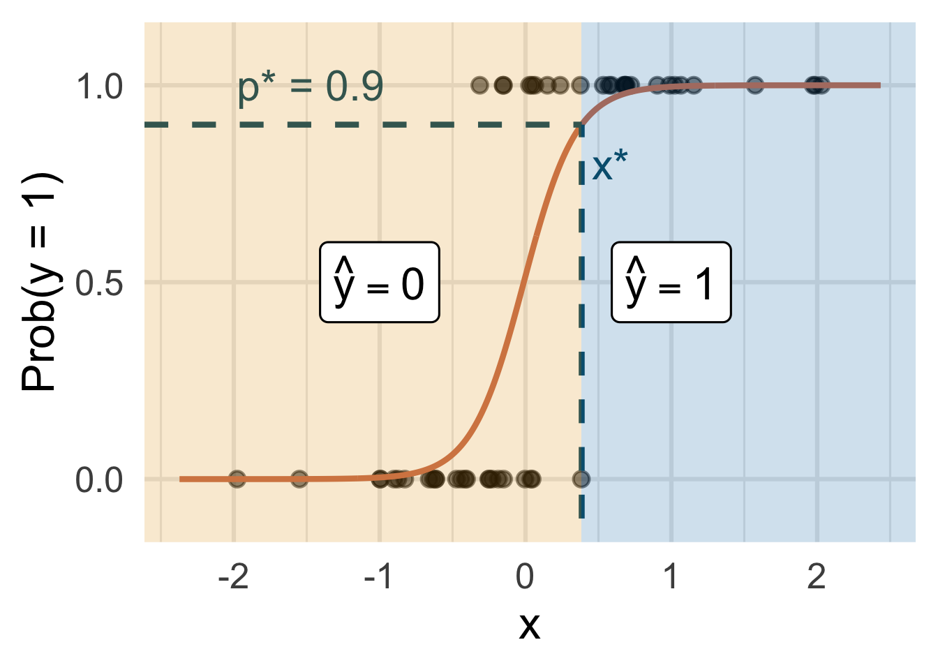
• if \(x_{\text{new}} \leq x^\star\), then \(\text{Prob}(y=1)\leq p^*\), so predict \(\widehat{y}=0\) for the new person
• if \(x_{\text{new}} > x^\star\), then \(\text{Prob}(y=1)> p^*\), so predict \(\widehat{y}=1\) for the new person.

Nothing special about one predictor…

Two numerical predictors and one binary outcome:

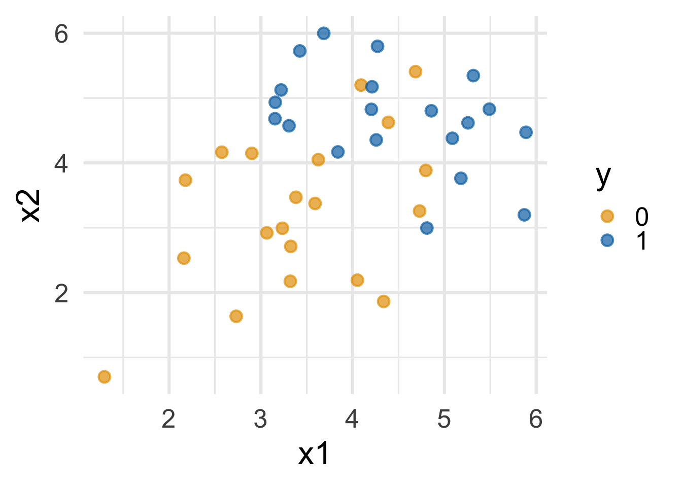
“Multiple” logistic regression

On the probability scale:

\[ \text{Prob}(y = 1) = \frac{e^{\beta_0+\beta_1x_1+\beta_2x_2+...+\beta_mx_m}}{1+e^{\beta_0+\beta_1x_1+\beta_2x_2+...+\beta_mx_m}}. \]

For the log-odds, a multiple linear regression:

\[ \log\left(\frac{p}{1-p}\right) = \beta_0+\beta_1x_1+\beta_2x_2+...+\beta_mx_m. \]

Decision boundary, again

It’s linear! Consider two numerical predictors:

• if new \((x_1,\,x_2)\) below, \(\text{Prob}(y=1)\leq p^*\) \(\rightarrow\) predict \(\widehat{y}=0\) for new observation
• if new \((x_1,\,x_2)\) above, \(\text{Prob}(y=1)> p^*\) \(\rightarrow\) predict \(\widehat{y}=1\) for new observation

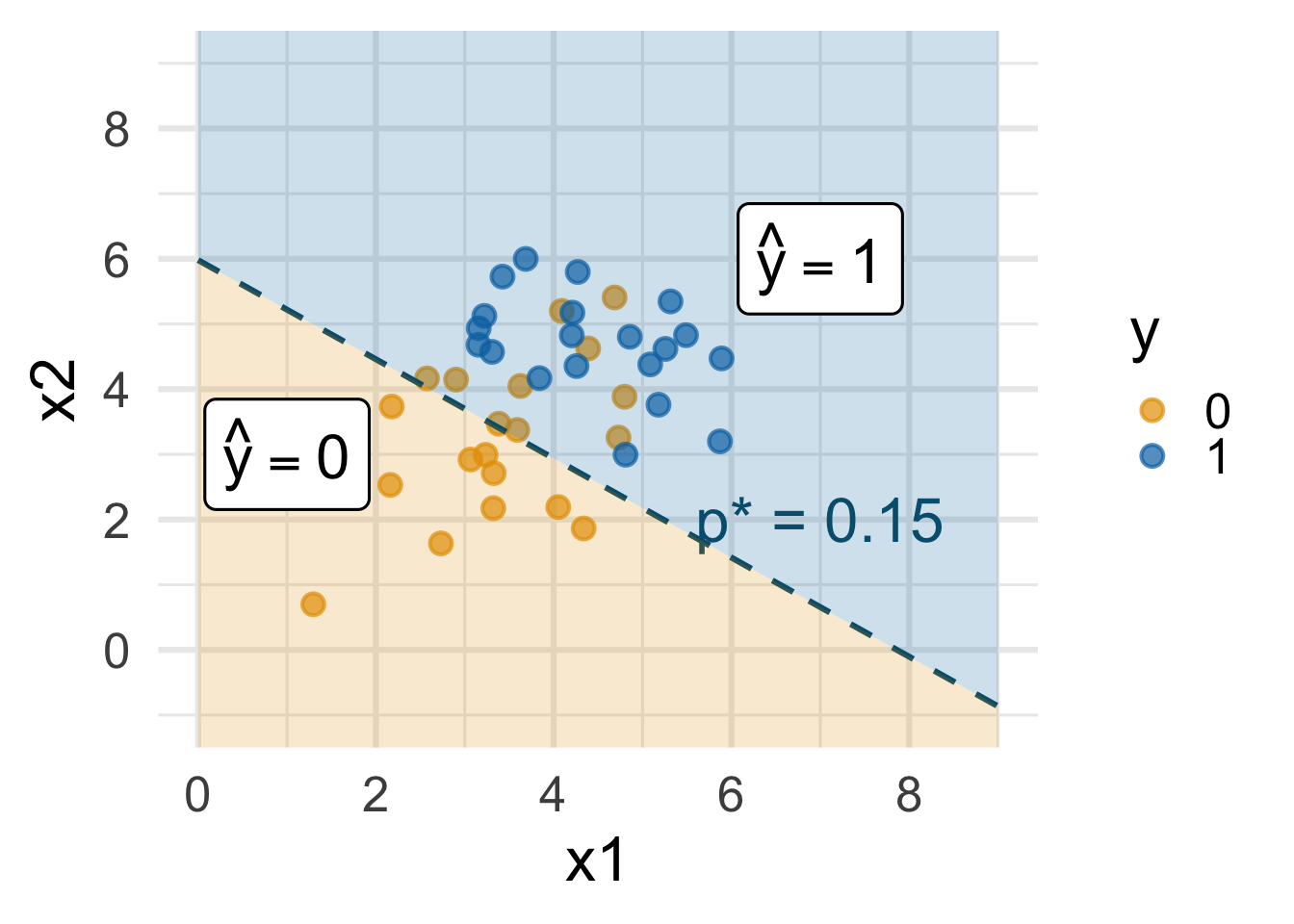
Decision boundary, again

It’s linear! Consider two numerical predictors:

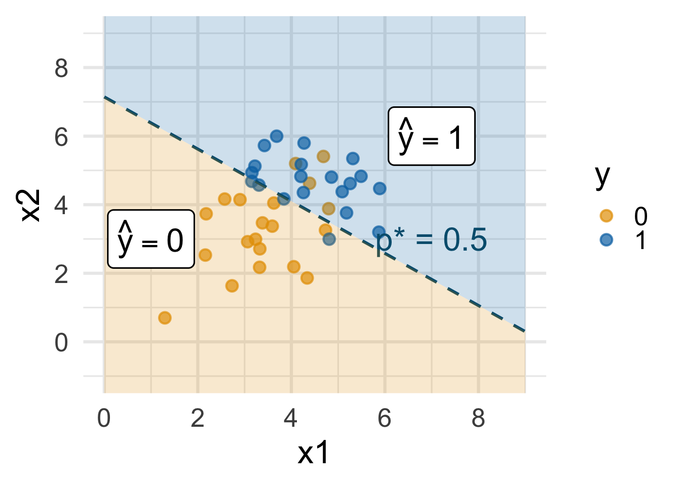
• if new \((x_1,\,x_2)\) below, \(\text{Prob}(y=1)\leq p^*\) \(\rightarrow\) predict \(\widehat{y}=0\) for new observation
• if new \((x_1,\,x_2)\) above, \(\text{Prob}(y=1)> p^*\) \(\rightarrow\) predict \(\widehat{y}=1\) for new observation

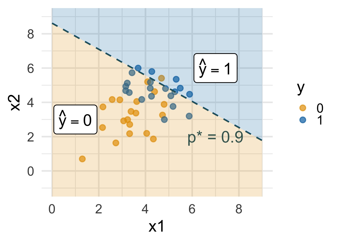
Decision boundary, again

It’s linear! Consider two numerical predictors:

• if new \((x_1,\,x_2)\) below, \(\text{Prob}(y=1)\leq p^*\) \(\rightarrow\) predict \(\widehat{y}=0\) for new observation
• if new \((x_1,\,x_2)\) above, \(\text{Prob}(y=1)> p^*\) \(\rightarrow\) predict \(\widehat{y}=1\) for new observation

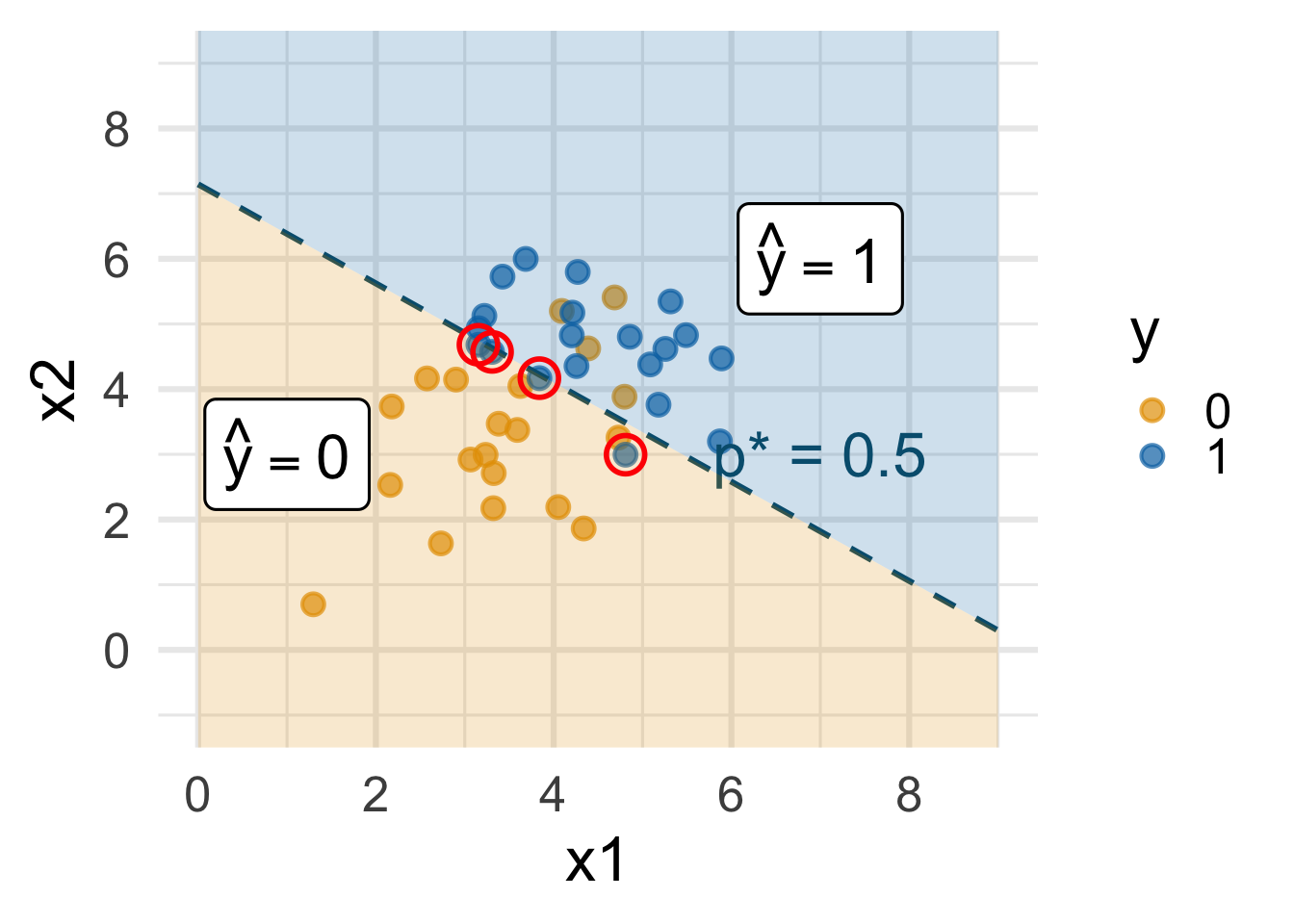
The classifier isn’t perfect

There are blue points in the orange region and oranges in the blue:

The classifier isn’t perfect

Blue points in the orange region: spam (1) emails misclassified as legit (0)

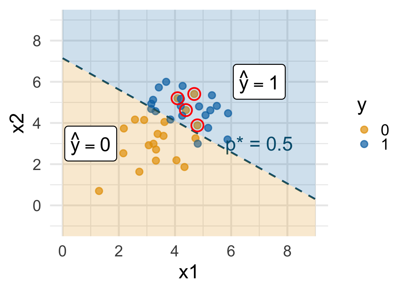
The classifier isn’t perfect

Orange points in the blue region: legit (0) emails misclassified as spam (1)

How do you pick the threshold?

To balance out the two kinds of errors:

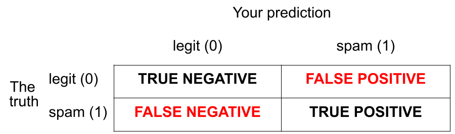
• High threshold >> Hard to classify as 1 >> FP less likely, FN more likely
• Low threshold >> Easy to classify as 1 >> FP more likely, FN less likely

Silly examples

• Set p* = 0

  • Classify every email as spam (1)
  • No false negatives, but a lot of false positives

• Set p* = 1

  • Classify every email as legit (0)
  • No false positives, but a lot of false negatives.

You pick a threshold in between to strike a balance. The exact number depends on context.

ae-13-spam-filter

• Go to your ae project in RStudio.

• If you haven’t yet done so, make sure all of your changes up to this point are committed and pushed, i.e., there’s nothing left in your Git pane.

• If you haven’t yet done so, click Pull to get today’s application exercise file: ae-13-spam-filter.qmd.

• Work through the application exercise in class, and render, commit, and push your edits.