Logistic regression

Lecture 20

Dr. Mine Çetinkaya-Rundel

Duke University
STA 199 - Fall 2025

November 6, 2025

Warm-up

Announcements

My Friday office hours extended – 12:45 - 3:00 PM in for this week
Project presentations: Hard stop at 5 minute mark! No limit on number of slides, but be mindful of how long it takes you to go through each.

Project questions

Focus: Can expand focus after research question, sure!
Citations: Don’t have to have them on slides and don’t need to say them out loud unless relevant to presentation, must include in writeup.
Vairble names: It’s ok to have some long variable names, but if you’re using them a lot in your code, make sure code is easy to follow.
Outliers: Evaluate if they’re genuinely influencing your model.
Grading: Rubric is in the milestone 6.
Categorical variables + summary stats: Correlation isn’t appropriate, report %s or make stacked bar plots.
There is no single correct number of graphs, tables, etc.
Review your website by clicking on the link from your repo.
Analysis writeup can be broken into multiple pieces with plots, tables, etc. sprinkled.
Who is grading? TAs and myself, I’ll be at (most of) the presentations.
When is it due?

Logistic regression

Packages

library(tidyverse) # data wrangling and visualization
library(tidymodels) # modeling
library(openintro) # emails data
library(fivethirtyeight) # movies data
library(palmerpenguins) # penguins data
library(ggthemes) # accessible color palettes

Thus far…

We have been studying regression:

What combinations of data types have we seen?
What did the picture look like?

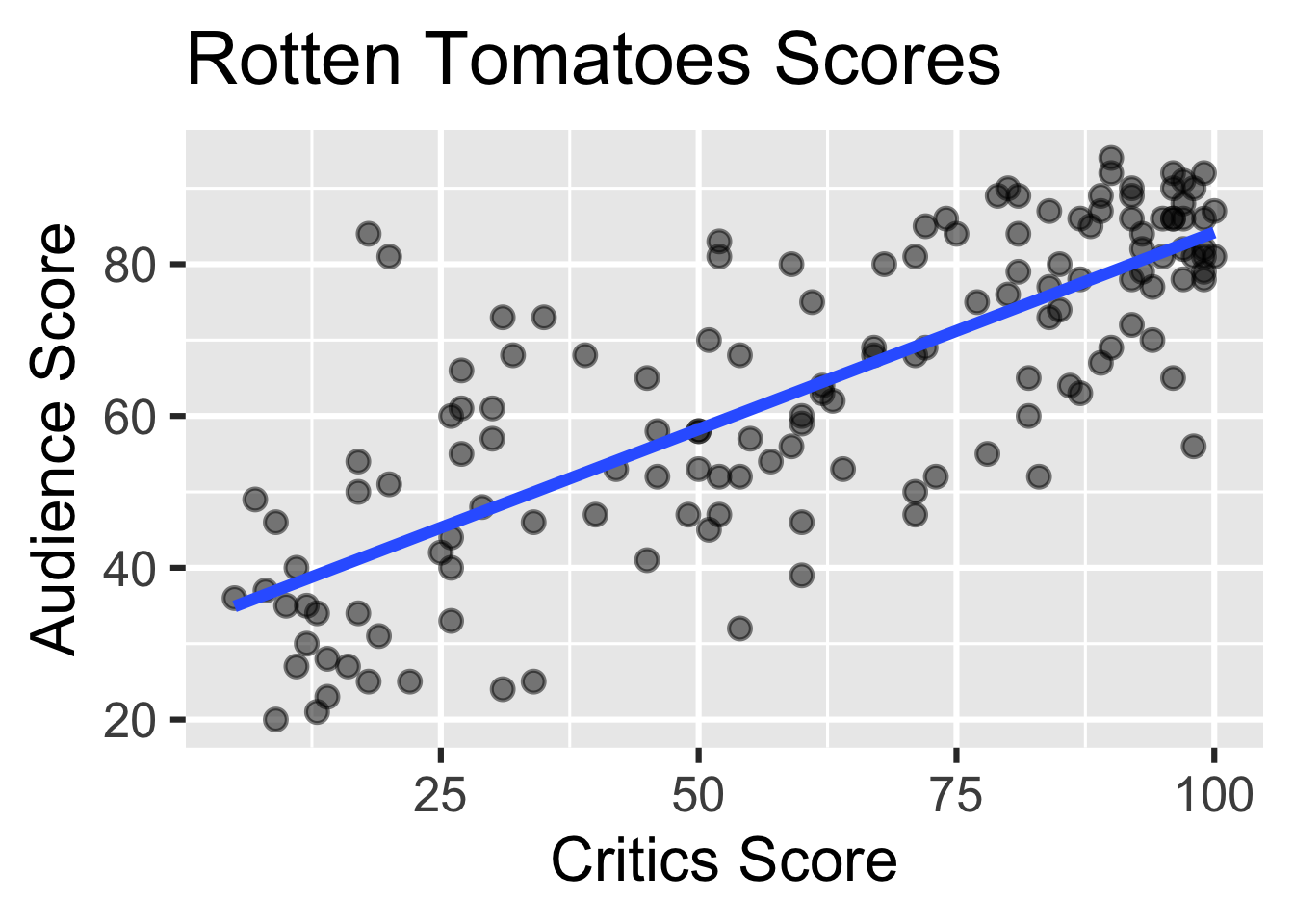
Recap: Simple linear regression

Numerical outcome and one numerical predictor:

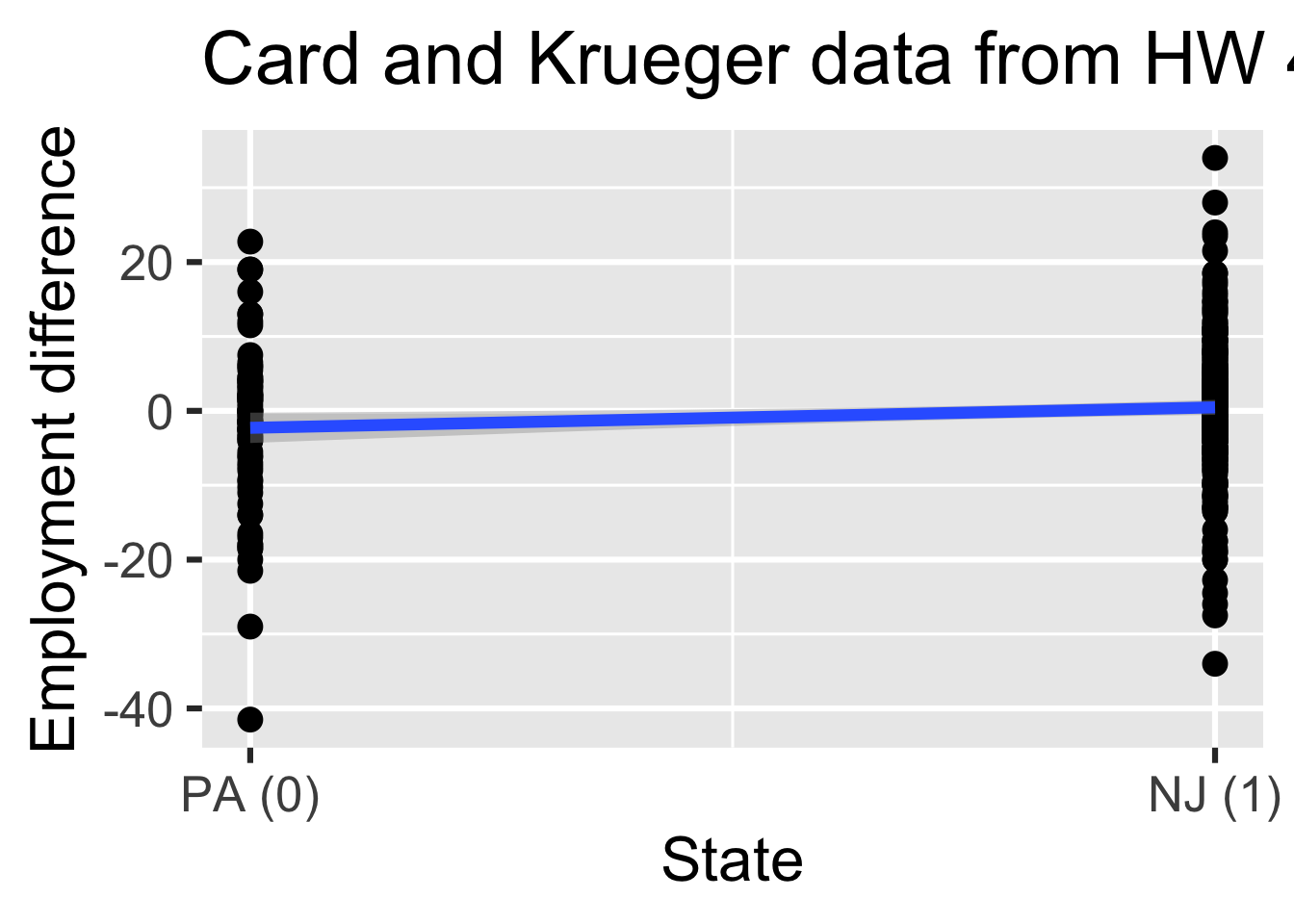
Recap: Simple linear regression

Numerical outcome and one categorical predictor (two levels):

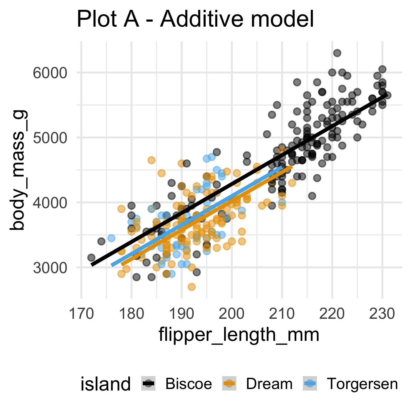
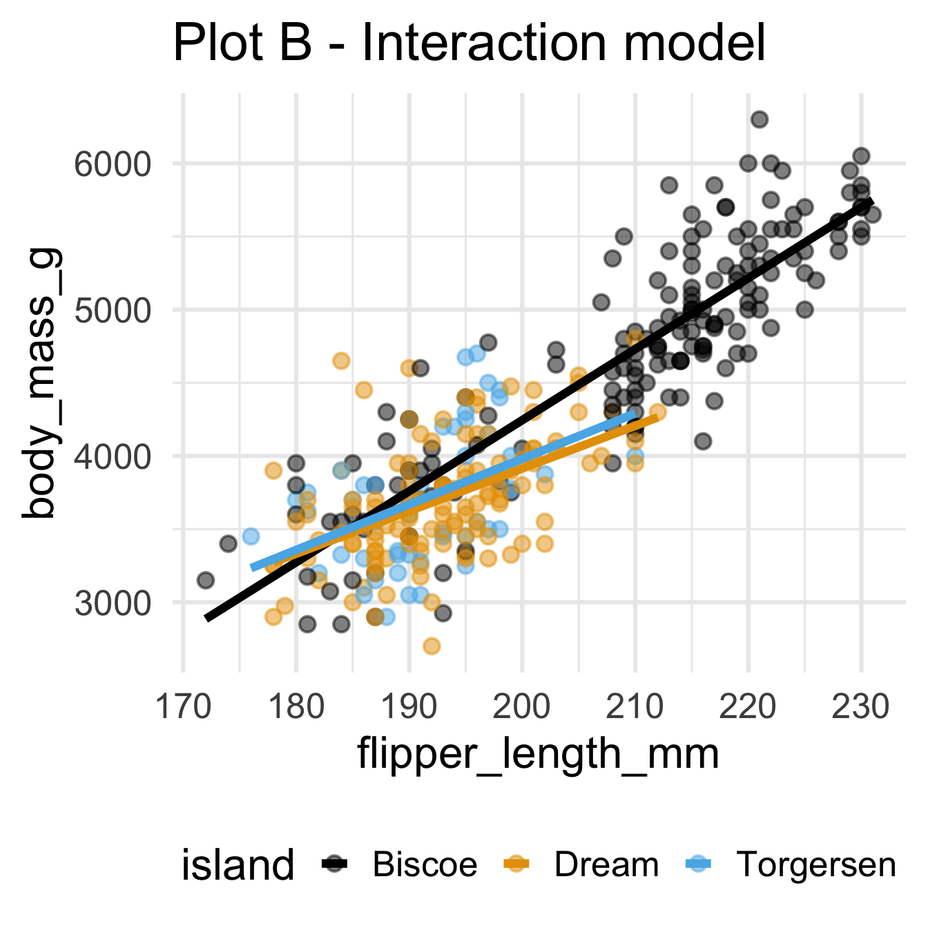
Recap: Multiple linear regression

Numerical outcome, numerical and categorical predictors:

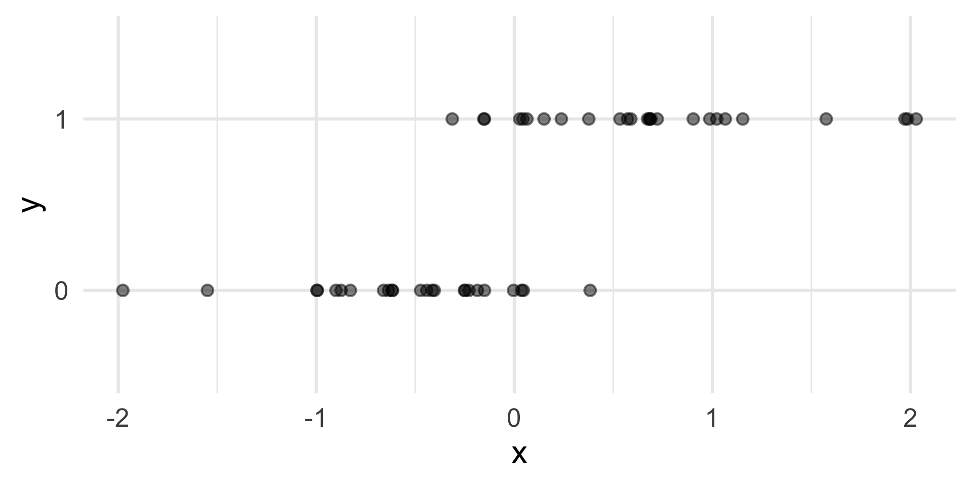
Today: a binary outcome

\[ y = \begin{cases} 1 & &&\text{eg. Yes, Win, True, Heads, Success}\\ 0 & &&\text{eg. No, Lose, False, Tails, Failure}. \end{cases} \]

Who cares?

If we can model the relationship between predictors (\(x\)) and a binary outcome (\(y\)), we can use the model to do a special kind of prediction called classification.

Example: Is the e-mail spam or not?

\[ \mathbf{x}: \text{word and character counts in an e-mail.} \]

\[ y = \begin{cases} 1 & \text{it's spam}\\ 0 & \text{it's legit} \end{cases} \]

Example: Is it cancer or not?

\[ \mathbf{x}: \text{features in a medical image.} \]

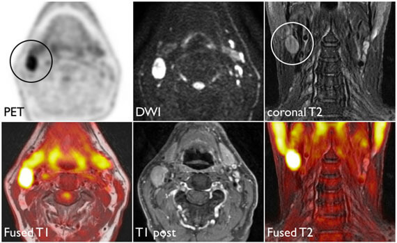
\[ y = \begin{cases} 1 & \text{it's cancer}\\ 0 & \text{it's healthy} \end{cases} \]

Example: Will they default?

\[ \mathbf{x}: \text{financial and demographic info about a loan applicant.} \]

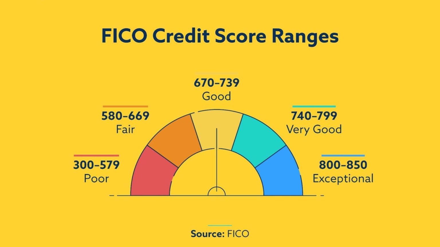
\[ y = \begin{cases} 1 & \text{applicant is at risk of defaulting on loan}\\ 0 & \text{applicant is safe} \end{cases} \]

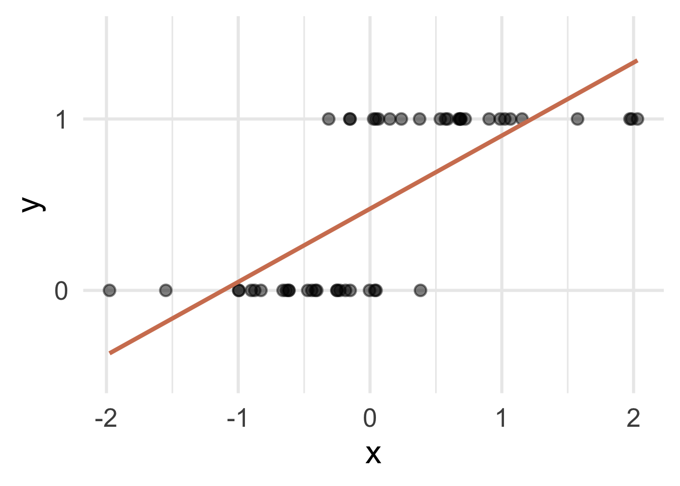
How do we model this type of data?

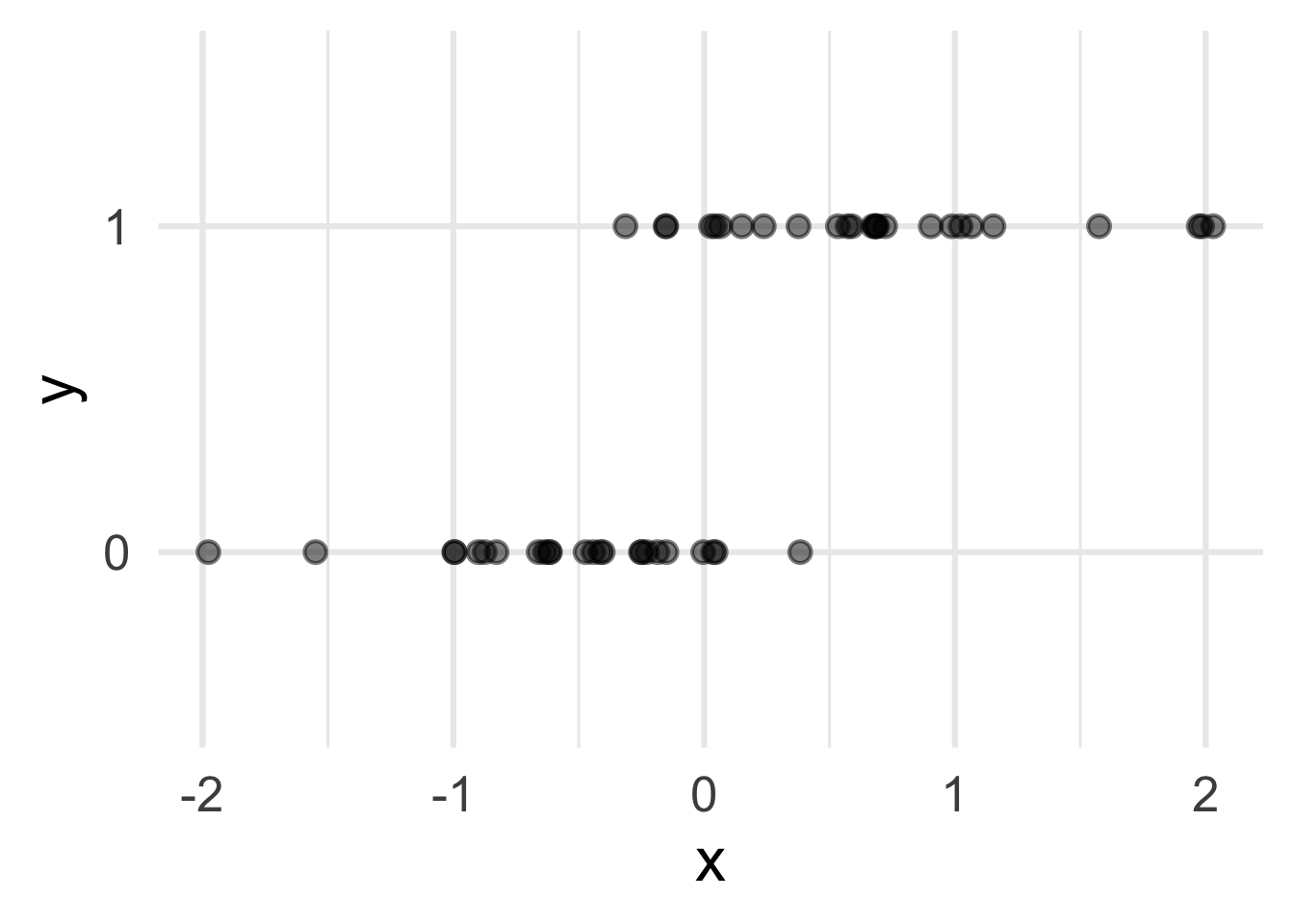
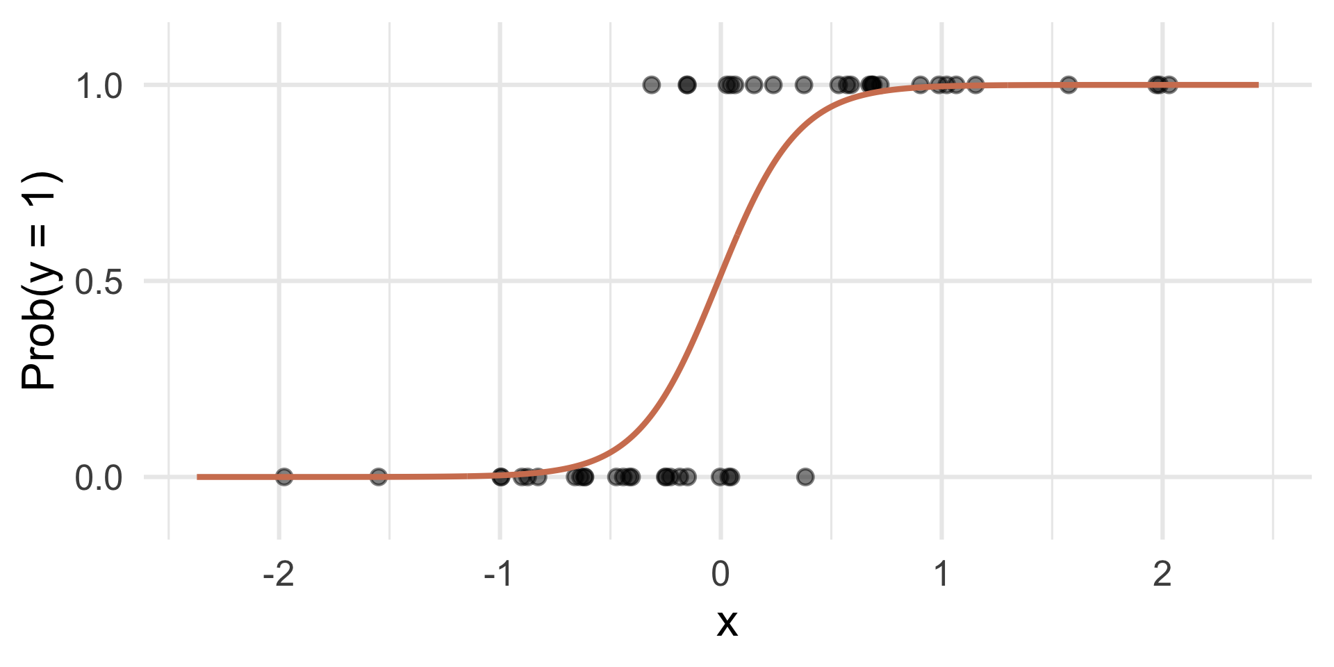
Straight line of best fit is a little silly

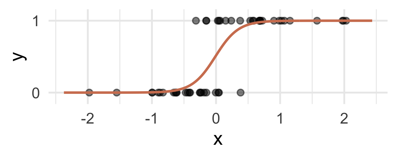
Instead: S-curve of best fit

Instead of modeling \(y\) directly, we model the probability that \(y=1\):

“Given new email, what’s the probability that it’s spam?’’
“Given new image, what’s the probability that it’s cancer?’’
“Given new loan application, what’s the probability that they default?’’

Why don’t we model y directly?

Recall regression with a numerical outcome:
- Our models do not output guarantees for \(y\), they output predictions that describe behavior on average
Similar when modeling a binary outcome:
- Our models cannot directly guarantee that \(y\) will be zero or one. The correct analog to “on average” for a 0/1 outcome is “what’s the probability?”

So, what is this S-curve, anyway?

It’s the logistic function:

\[ \text{Prob}(y = 1) = \frac{e^{\beta_0+\beta_1x}}{1+e^{\beta_0+\beta_1x}}. \]

If you set \(p = \text{Prob}(y = 1)\) and do some algebra, you get the simple linear model for the log-odds:

\[ \log\left(\frac{p}{1-p}\right) = \beta_0+\beta_1x. \]

This is called the logistic regression model.

Log-odds?

\(p = \text{Prob}(y = 1)\) is a probability. A number between 0 and 1
\(p / (1 - p)\) is the odds. A number between 0 and \(\infty\)

“The odds of this lecture going well are 10 to 1.”

The log odds \(\log(p / (1 - p))\) is a number between \(-\infty\) and \(\infty\), which is suitable for the linear model.

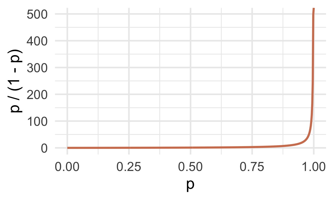
Probability to odds

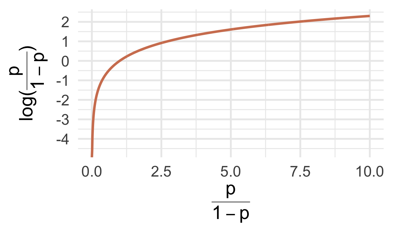
Odds to log odds

Participate 📱💻

If \(p\) is the probability of success, what is the following called:

\[ \frac{p}{1-p} \]

Probability of failure
Odds of failure
Odds of success
Log-odds of success

Scan the QR code or go to app.wooclap.com/sta199. Log in with your Duke NetID.

Logistic regression

\[ \log\left(\frac{p}{1-p}\right) = \beta_0+\beta_1x. \]

The logit function \(\log(p / (1-p))\) is an example of a link function that transforms the linear model to have an appropriate range
This is an example of a generalized linear model

Estimation

We estimate the parameters \(\beta_0\) (intercept) and \(\beta_1\) (slope) using maximum likelihood (don’t worry about it) to get the “best fitting” S-curve
The fitted model is

\[ \log\left(\frac{\widehat{p}}{1-\widehat{p}}\right) = b_0+b_1x. \]

Today’s data

email |>
  select(c(spam, dollar, viagra, winner, password, exclaim_mess)) |>
  glimpse()

Rows: 3,921
Columns: 6
$ spam         <fct> 0, 0, 0, 0, 0, 0, 0, 0, 0, 0, 0, 0, 0, 0, 0, 0,…
$ dollar       <dbl> 0, 0, 4, 0, 0, 0, 0, 0, 0, 0, 0, 0, 0, 0, 2, 0,…
$ viagra       <dbl> 0, 0, 0, 0, 0, 0, 0, 0, 0, 0, 0, 0, 0, 0, 0, 0,…
$ winner       <fct> no, no, no, no, no, no, no, no, no, no, no, no,…
$ password     <dbl> 0, 0, 0, 0, 2, 2, 0, 0, 0, 0, 0, 0, 0, 0, 0, 0,…
$ exclaim_mess <dbl> 0, 1, 6, 48, 1, 1, 1, 18, 1, 0, 2, 1, 0, 10, 4,…

Fitting a logistic model

logistic_fit <- logistic_reg() |>
  fit(spam ~ exclaim_mess, data = email)

tidy(logistic_fit)

# A tibble: 2 × 5
  term          estimate std.error statistic p.value
  <chr>            <dbl>     <dbl>     <dbl>   <dbl>
1 (Intercept)  -2.27      0.0553     -41.1     0    
2 exclaim_mess  0.000272  0.000949     0.287   0.774

Fitted equation for the log-odds:

\[ \log\left(\frac{\hat{p}}{1-\hat{p}}\right) = -2.27 + 0.000272\times exclaim~mess \]

Interpreting the intercept

If exclaim_mess = 0, then

\[ \hat{p}=\widehat{P(y=1)}=\frac{e^{-2.27}}{1+e^{-2.27}}\approx 0.09. \]

So, an email with no exclamation marks has a 9% chance of being spam.

Interpreting the slope is tricky

Recall:

\[ \log\left(\frac{\widehat{p}}{1-\widehat{p}}\right) = b_0+b_1x. \]

Alternatively:

\[ \frac{\widehat{p}}{1-\widehat{p}} = e^{b_0+b_1x} = \color{blue}{e^{b_0}e^{b_1x}} . \]

If \(x\) is higher by one unit, we have:

\[ \frac{\widehat{p}}{1-\widehat{p}} = e^{b_0}e^{b_1(x+1)} = e^{b_0}e^{b_1x+b_1} = {\color{blue}{e^{b_0}e^{b_1x}}}{\color{red}{e^{b_1}}} . \]

A one unit increase in \(x\) is associated with a change in odds by a factor of \(e^{b_1}\). Helpful! 🙄

Back to the example…

\[ \log\left(\frac{\hat{p}}{1-\hat{p}}\right) = -2.27 + 0.000272\times exclaim~mess \]

Emails with one additional exclamation point are predicted to have odds of being spam that are higher by a factor of \(e^{0.000272}\approx 1.000272\), on average.

Classification
(logistic regression by another name…)

Step 1: fit the model

Select a number \(0 < p^* < 1\):

if \(\text{Prob}(y=1)\leq p^*\), then predict \(\widehat{y}=0\)
if \(\text{Prob}(y=1)> p^*\), then predict \(\widehat{y}=1\).

Step 2: pick a threshold

Select a number \(0 < p^* < 1\):

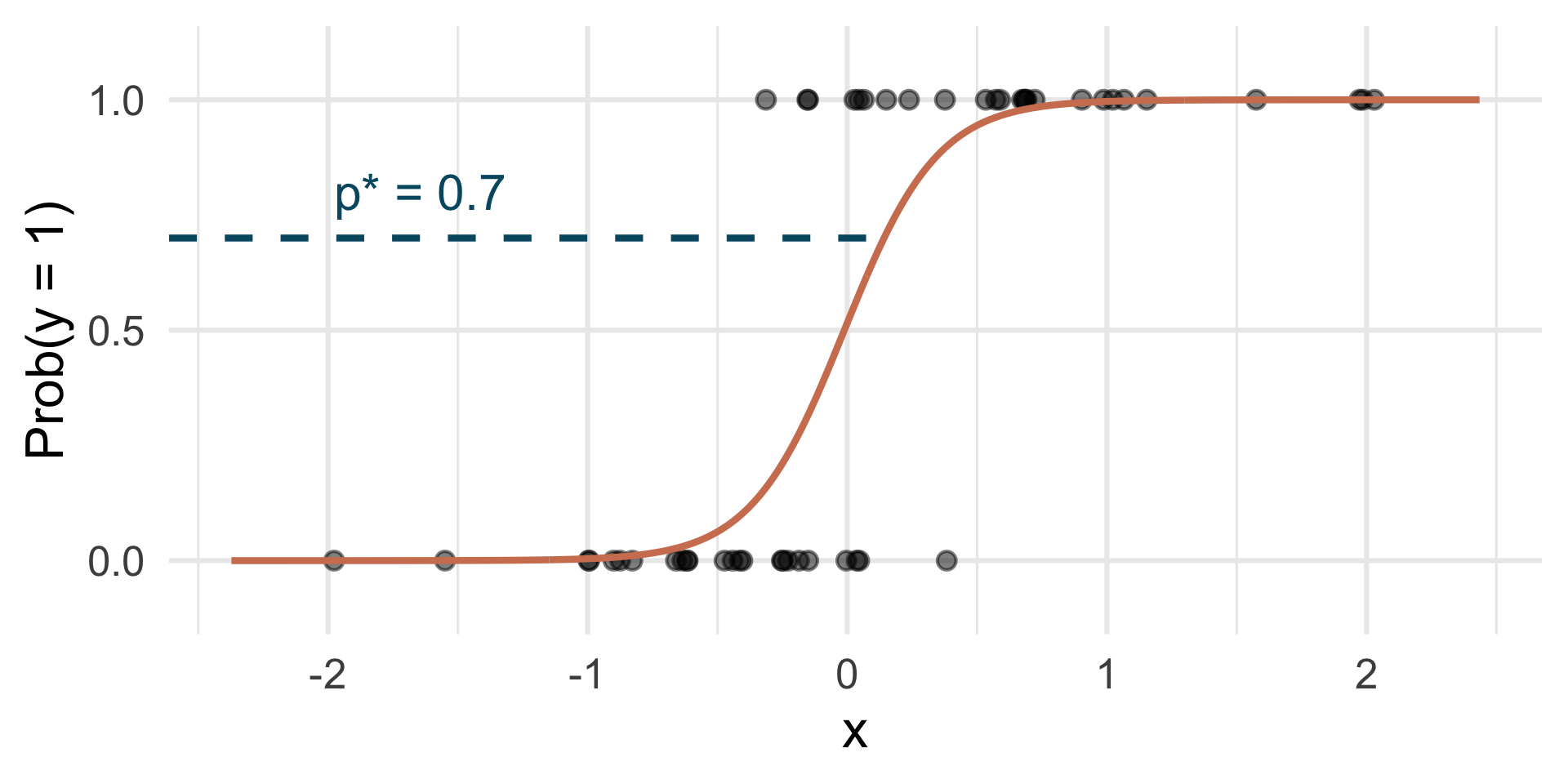
if \(\text{Prob}(y=1)\leq p^*\), then predict \(\widehat{y}=0\)
if \(\text{Prob}(y=1)> p^*\), then predict \(\widehat{y}=1\).

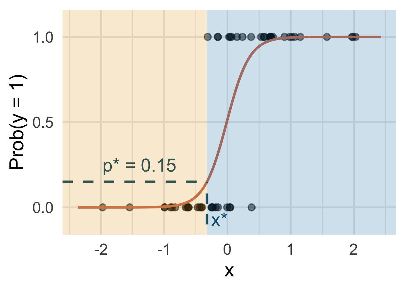
Step 3: find the “decision boundary”

Solve for the x-value that matches the threshold:

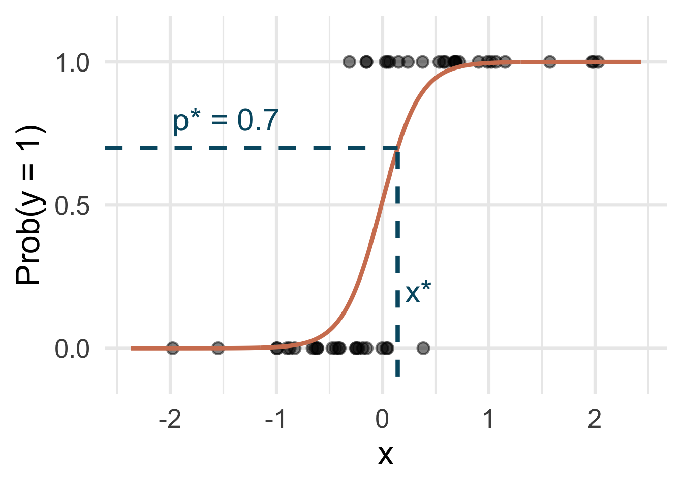
if \(\text{Prob}(y=1)\leq p^*\), then predict \(\widehat{y}=0\)
if \(\text{Prob}(y=1)> p^*\), then predict \(\widehat{y}=1\).

Step 4: classify a new arrival

A new person shows up with \(x_{\text{new}}\). Which side of the boundary are they on?

if \(x_{\text{new}} \leq x^\star\), then \(\text{Prob}(y=1)\leq p^*\), so predict \(\widehat{y}=0\) for the new person
if \(x_{\text{new}} > x^\star\), then \(\text{Prob}(y=1)> p^*\), so predict \(\widehat{y}=1\) for the new person.

Let’s change the threshold

A new person shows up with \(x_{\text{new}}\). Which side of the boundary are they on?

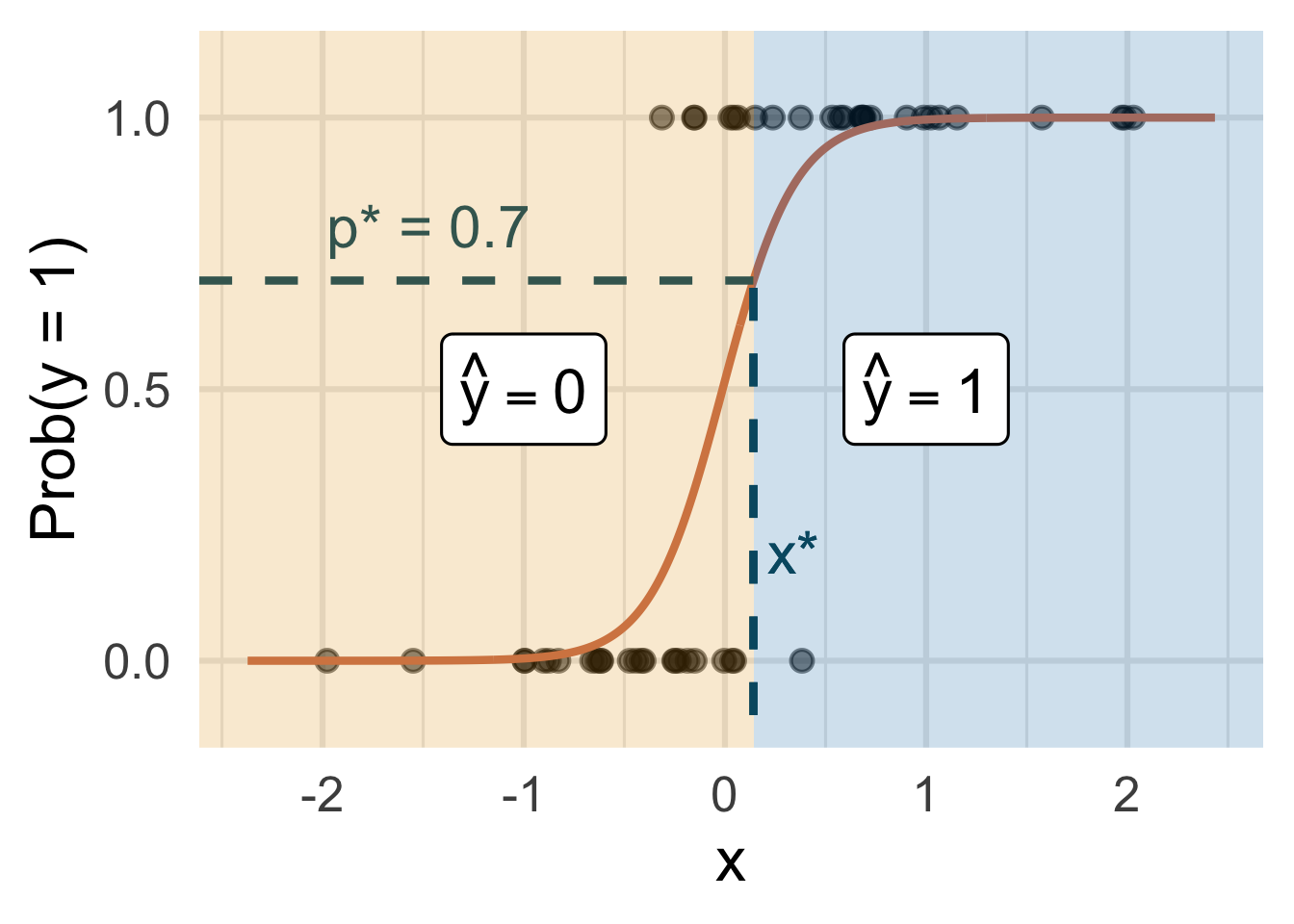
if \(x_{\text{new}} \leq x^\star\), then \(\text{Prob}(y=1)\leq p^*\), so predict \(\widehat{y}=0\) for the new person
if \(x_{\text{new}} > x^\star\), then \(\text{Prob}(y=1)> p^*\), so predict \(\widehat{y}=1\) for the new person.

Let’s change the threshold

A new person shows up with \(x_{\text{new}}\). Which side of the boundary are they on?

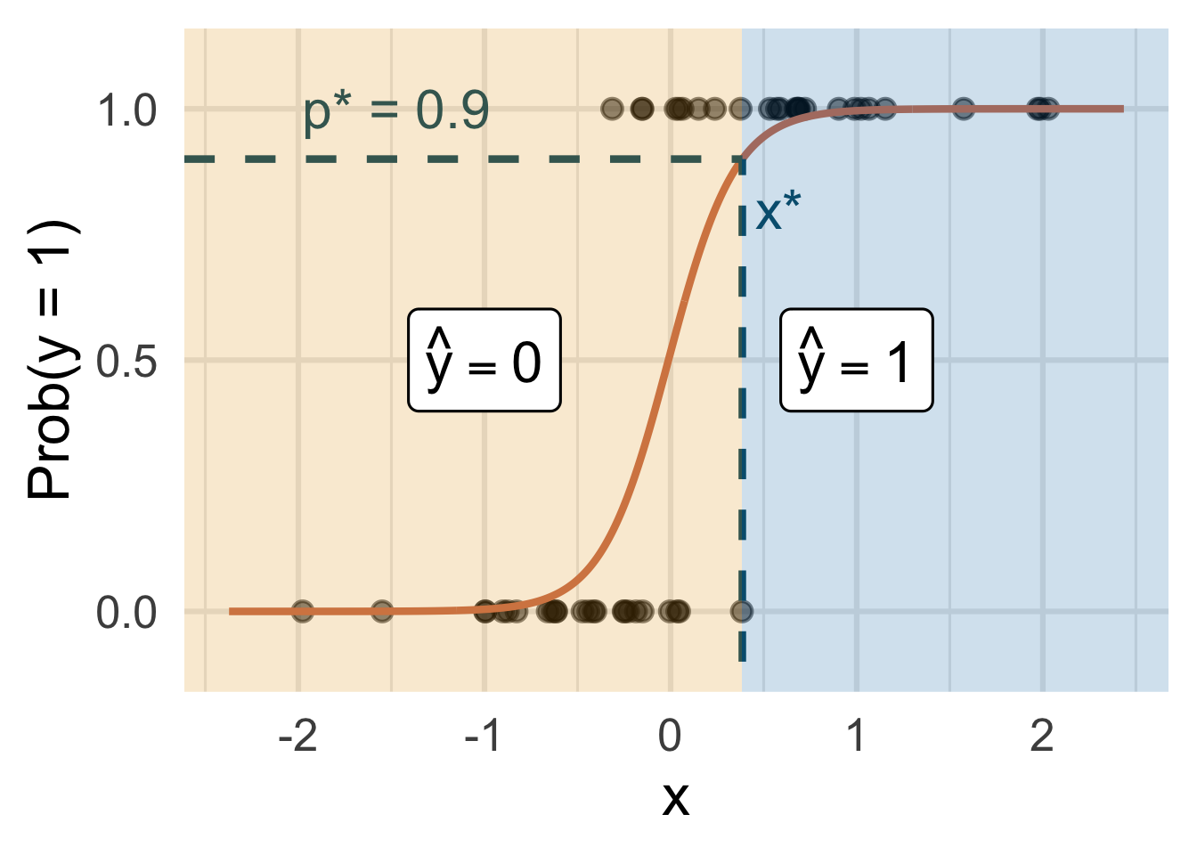
if \(x_{\text{new}} \leq x^\star\), then \(\text{Prob}(y=1)\leq p^*\), so predict \(\widehat{y}=0\) for the new person
if \(x_{\text{new}} > x^\star\), then \(\text{Prob}(y=1)> p^*\), so predict \(\widehat{y}=1\) for the new person.

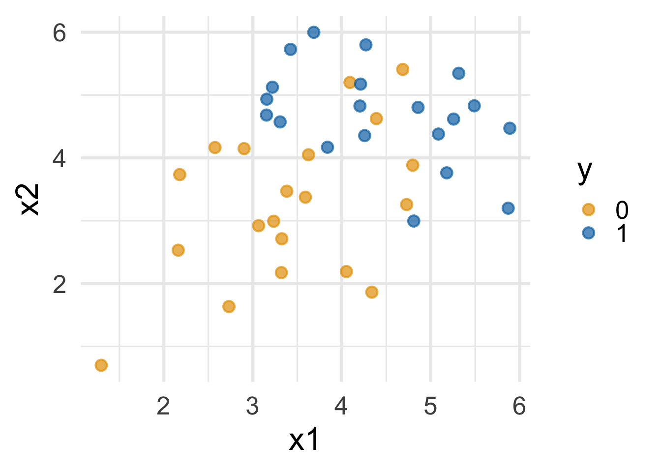
Nothing special about one predictor…

Two numerical predictors and one binary outcome:

“Multiple” logistic regression

On the probability scale:

\[ \text{Prob}(y = 1) = \frac{e^{\beta_0+\beta_1x_1+\beta_2x_2+...+\beta_mx_m}}{1+e^{\beta_0+\beta_1x_1+\beta_2x_2+...+\beta_mx_m}}. \]

For the log-odds, a multiple linear regression:

\[ \log\left(\frac{p}{1-p}\right) = \beta_0+\beta_1x_1+\beta_2x_2+...+\beta_mx_m. \]

Decision boundary, again

It’s linear! Consider two numerical predictors:

if new \((x_1,\,x_2)\) below, \(\text{Prob}(y=1)\leq p^*\) \(\rightarrow\) predict \(\widehat{y}=0\) for new observation
if new \((x_1,\,x_2)\) above, \(\text{Prob}(y=1)> p^*\) \(\rightarrow\) predict \(\widehat{y}=1\) for new observation

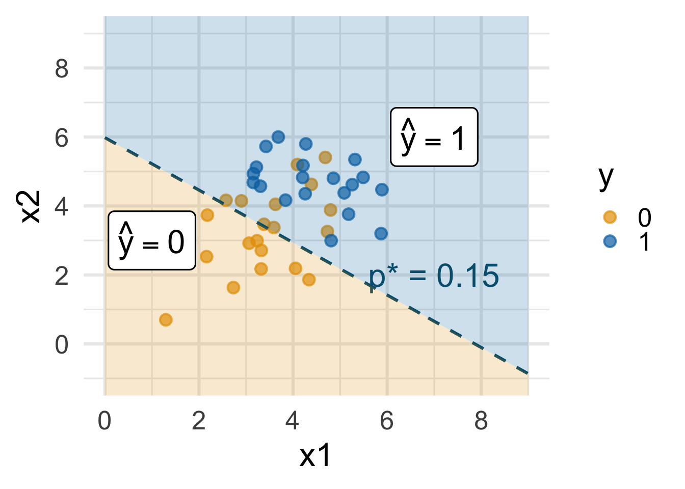
Decision boundary, again

It’s linear! Consider two numerical predictors:

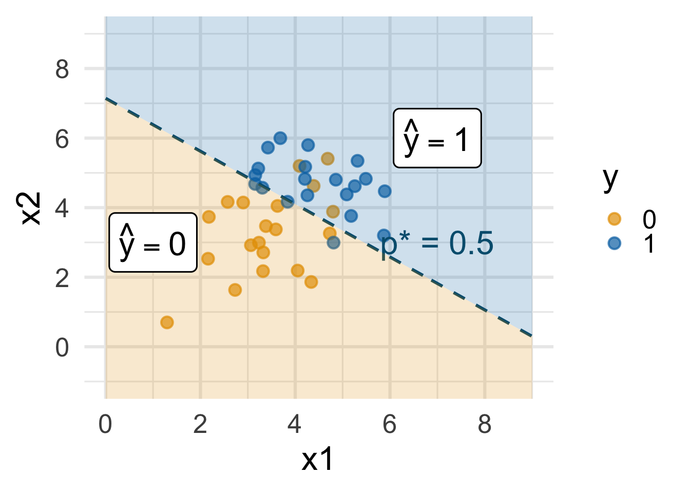
if new \((x_1,\,x_2)\) below, \(\text{Prob}(y=1)\leq p^*\) \(\rightarrow\) predict \(\widehat{y}=0\) for new observation
if new \((x_1,\,x_2)\) above, \(\text{Prob}(y=1)> p^*\) \(\rightarrow\) predict \(\widehat{y}=1\) for new observation

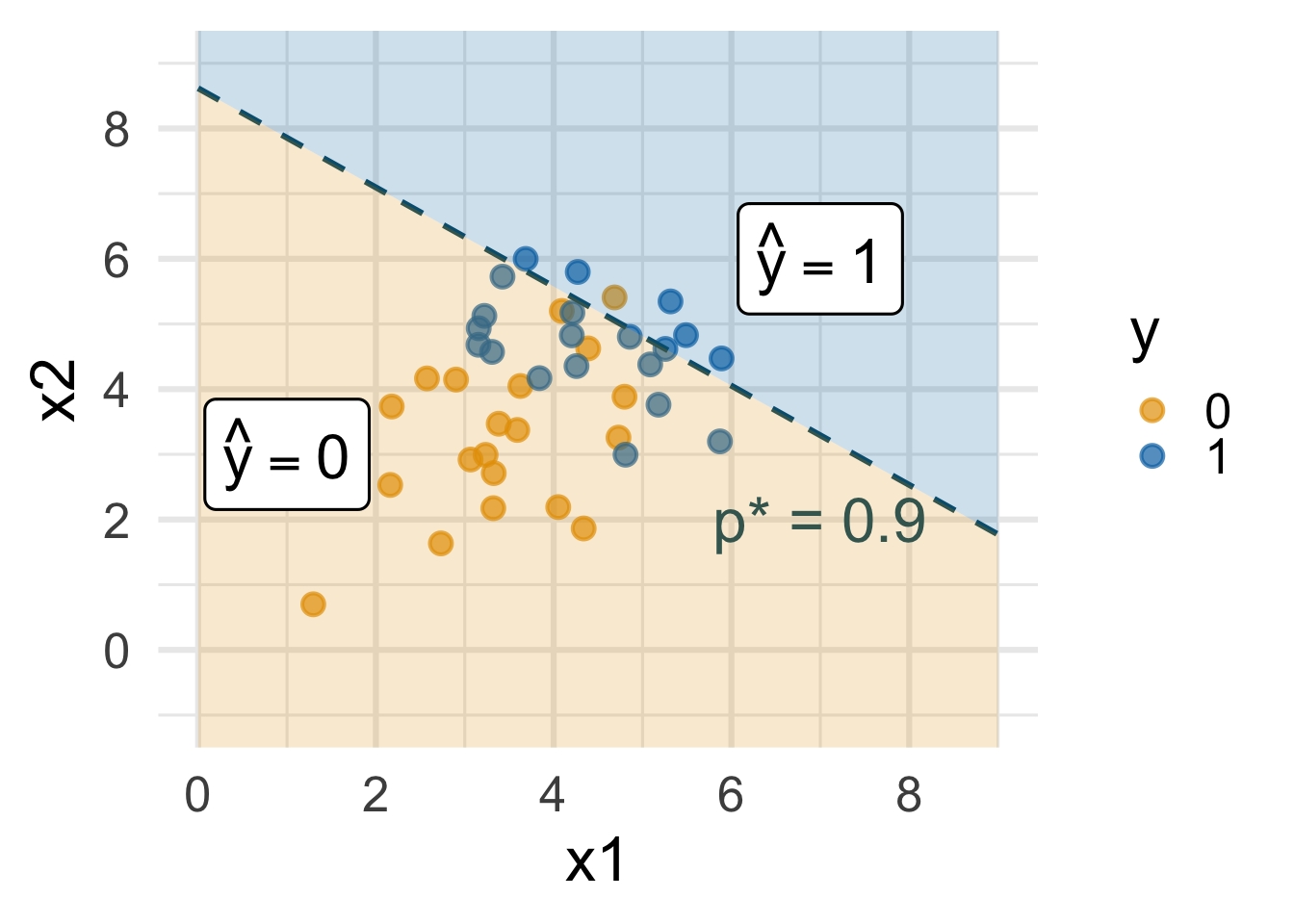
Decision boundary, again

It’s linear! Consider two numerical predictors:

if new \((x_1,\,x_2)\) below, \(\text{Prob}(y=1)\leq p^*\) \(\rightarrow\) predict \(\widehat{y}=0\) for new observation
if new \((x_1,\,x_2)\) above, \(\text{Prob}(y=1)> p^*\) \(\rightarrow\) predict \(\widehat{y}=1\) for new observation

The classifier isn’t perfect

There are blue points in the orange region and oranges in the blue:

The classifier isn’t perfect

Blue points in the orange region: spam (1) emails misclassified as legit (0)

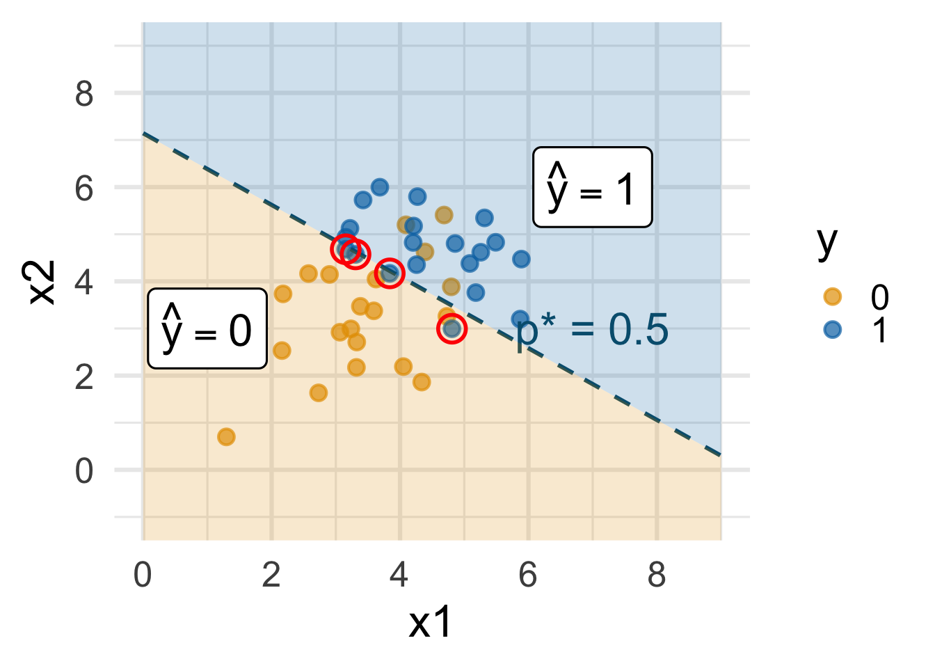
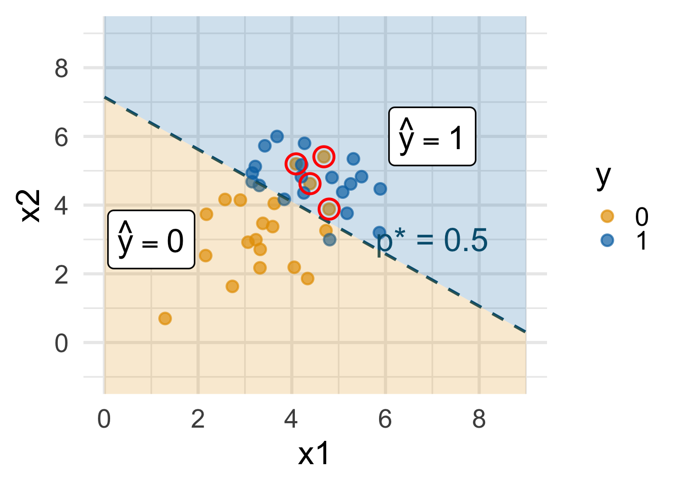
The classifier isn’t perfect

Orange points in the blue region: legit (0) emails misclassified as spam (1)

How do you pick the threshold?

To balance out the two kinds of errors:

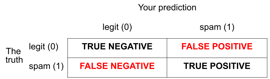
High threshold >> Hard to classify as 1 >> FP less likely, FN more likely
Low threshold >> Easy to classify as 1 >> FP more likely, FN less likely

Silly examples

Set p* = 0
- Classify every email as spam (1)
- No false negatives, but a lot of false positives
Set p* = 1
- Classify every email as legit (0)
- No false positives, but a lot of false negatives.

You pick a threshold in between to strike a balance. The exact number depends on context.

ae-13-spam-filter

Go to your ae project in RStudio.
If you haven’t yet done so, make sure all of your changes up to this point are committed and pushed, i.e., there’s nothing left in your Git pane.
If you haven’t yet done so, click Pull to get today’s application exercise file: ae-13-spam-filter.qmd.
Work through the application exercise in class, and render, commit, and push your edits.

Logistic regression

Warm-up

Announcements

Project questions

Logistic regression

Packages

Thus far…

Recap: Simple linear regression

Recap: Simple linear regression

Recap: Multiple linear regression

Today: a binary outcome

Who cares?

Example: Is the e-mail spam or not?

Example: Is it cancer or not?

Example: Will they default?

How do we model this type of data?

Straight line of best fit is a little silly

Instead: S-curve of best fit

Why don’t we model y directly?

So, what is this S-curve, anyway?

Log-odds?

Probability to odds

Odds to log odds

Participate 📱💻

Logistic regression

Estimation

Today’s data

Fitting a logistic model

Interpreting the intercept

Interpreting the slope is tricky

Back to the example…

Classification (logistic regression by another name…)

Step 1: fit the model

Step 2: pick a threshold

Step 3: find the “decision boundary”

Step 4: classify a new arrival

Let’s change the threshold

Let’s change the threshold

Nothing special about one predictor…

“Multiple” logistic regression

Decision boundary, again

Decision boundary, again

Decision boundary, again

The classifier isn’t perfect

The classifier isn’t perfect

The classifier isn’t perfect

How do you pick the threshold?

Silly examples

ae-13-spam-filter

Classification
(logistic regression by another name…)