Exploratory data analysis II

Lecture 6

Author

Affiliation

Dr. Mine Çetinkaya-Rundel

Duke University
STA 199 - Fall 2025

Published

September 11, 2025

Warm-up

While you wait: Participate 📱💻

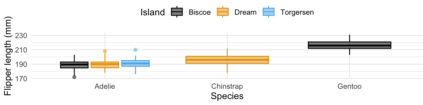
Which of the following is false about the following plot and the code that produced it?

Scan the QR code or go to app.wooclap.com/sta199. Log in with your Duke NetID.

There are no Chinstrap or Gentoo penguins on Torgersen Island.
legend.position = "bottom" is set in the theme() layer.
The same variable is mapped to both color and fill.
group_by(species) is used to create the boxplots. [*]
A Biscoe island penguin with a flipper length of 190 mm must be an Adélie.

Reminder: Code style and readability

Plots should include an informative title, axes and legends should have human-readable labels, and careful consideration should be given to aesthetic choices.
Code should follow the tidyverse style (style.tidyverse.org) Particularly,
- space before and line breaks after each + when building a ggplot
- space before and line breaks after each |> in a data transformation pipeline
- code should be properly indented
- spaces around = signs and spaces after commas
All code should be visible in the PDF output, i.e., should not run off the page on the PDF. Long lines that run off the page should be split across multiple lines with line breaks. Tip: Haikus not novellas when writing code!
Whydowecareaboutthestyleandreadabilityofyourcode? \(\rightarrow\) Why do we care about the style and readability of your code?
Je voudrais un cafe \(\rightarrow\) Je voudrais un café

`gerrymander`

Packages

For the data: usdata

library(usdata)

For the analysis: tidyverse and ggthemes

library(tidyverse)
library(ggthemes)

From the AE

Is a Congressional District more likely to have high prevalence of gerrymandering if a Democrat was able to flip the seat in the 2018 election?

ggplot(
  gerrymander, 
  aes(x = flip18, fill = gerry)
  ) +
  geom_bar(position = "fill")

gerrymander |>
  count(flip18, gerry) |>
  group_by(flip18) |>
  mutate(prop = n / sum(n))

# A tibble: 8 × 4
# Groups:   flip18 [3]
  flip18 gerry     n  prop
   <dbl> <fct> <int> <dbl>
1     -1 low       2 0.4  
2     -1 mid       3 0.6  
3      0 low      52 0.133
4      0 mid     242 0.617
5      0 high     98 0.25 
6      1 low       8 0.211
7      1 mid      25 0.658
8      1 high      5 0.132

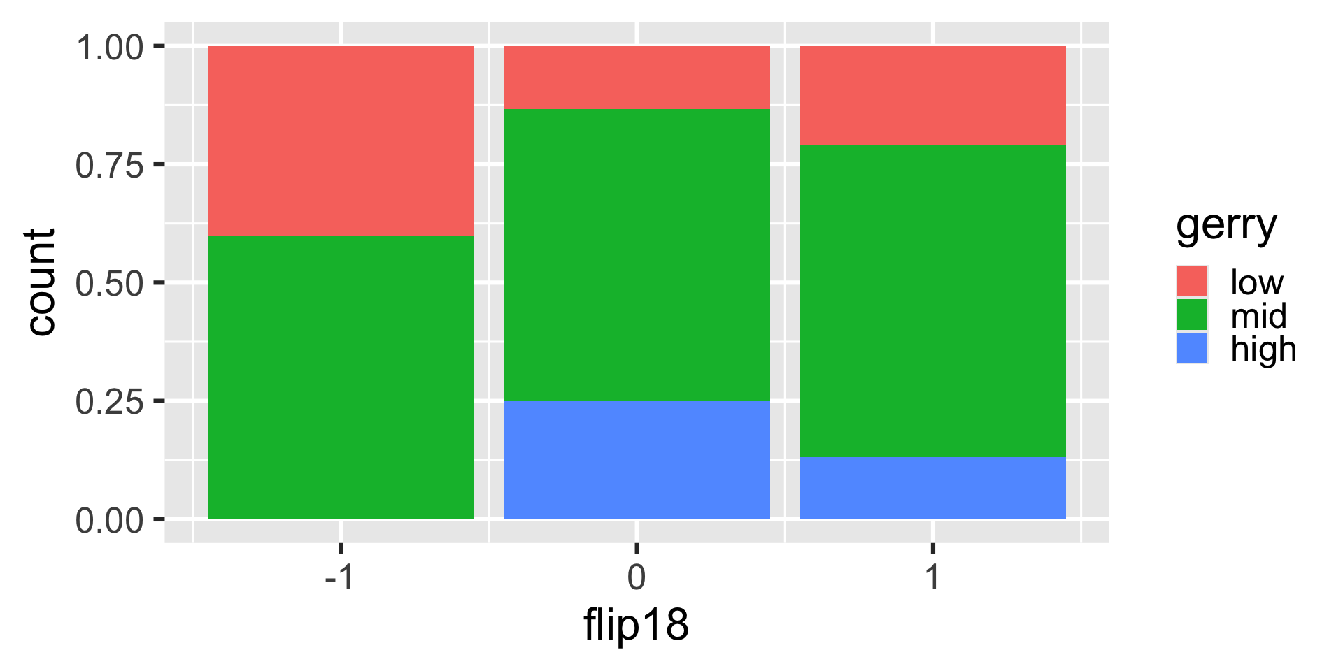
`group_by()`, `summarize()`, `count()`

What does `group_by()` do?

What does group_by() do in the following pipeline?

gerrymander |>
  count(flip18, gerry) |>
  group_by(flip18) |>
  mutate(prop = n / sum(n))

# A tibble: 8 × 4
# Groups:   flip18 [3]
  flip18 gerry     n  prop
   <dbl> <fct> <int> <dbl>
1     -1 low       2 0.4  
2     -1 mid       3 0.6  
3      0 low      52 0.133
4      0 mid     242 0.617
5      0 high     98 0.25 
6      1 low       8 0.211
7      1 mid      25 0.658
8      1 high      5 0.132

Let’s simplify!

What does group_by() do in the following pipeline?

gerrymander |>
  group_by(state) |>
  summarize(mean_trump16 = mean(trump16))

# A tibble: 50 × 2
   state mean_trump16
   <chr>        <dbl>
 1 AK            52.8
 2 AL            62.6
 3 AR            60.9
 4 AZ            46.9
 5 CA            31.7
 6 CO            43.6
 7 CT            41.0
 8 DE            41.9
 9 FL            47.9
10 GA            51.3
# ℹ 40 more rows

`group_by()`

Group by converts a data frame to a grouped data frame, where subsequent operations are performed once per group
ungroup() removes grouping

gerrymander |>
  group_by(state) |>
  ungroup()

# A tibble: 435 × 12
   district last_name first_name party16 clinton16 trump16 dem16 state
   <chr>    <chr>     <chr>      <chr>       <dbl>   <dbl> <dbl> <chr>
 1 AK-AL    Young     Don        R            37.6    52.8     0 AK   
 2 AL-01    Byrne     Bradley    R            34.1    63.5     0 AL   
 3 AL-02    Roby      Martha     R            33      64.9     0 AL   
 4 AL-03    Rogers    Mike D.    R            32.3    65.3     0 AL   
 5 AL-04    Aderholt  Rob        R            17.4    80.4     0 AL   
 6 AL-05    Brooks    Mo         R            31.3    64.7     0 AL   
 7 AL-06    Palmer    Gary       R            26.1    70.8     0 AL   
 8 AL-07    Sewell    Terri      D            69.8    28.6     1 AL   
 9 AR-01    Crawford  Rick       R            30.2    65       0 AR   
10 AR-02    Hill      French     R            41.7    52.4     0 AR   
# ℹ 425 more rows
# ℹ 4 more variables: party18 <chr>, dem18 <dbl>, flip18 <dbl>,
#   gerry <fct>

`group_by() |> summarize()`

A common pipeline is group_by() and then summarize() to calculate summary statistics for each group:

gerrymander |>
  group_by(state) |>
  summarize(
    mean_trump16 = mean(trump16),
    median_trump16 = median(trump16)
  )

# A tibble: 50 × 3
   state mean_trump16 median_trump16
   <chr>        <dbl>          <dbl>
 1 AK            52.8           52.8
 2 AL            62.6           64.9
 3 AR            60.9           63.0
 4 AZ            46.9           47.7
 5 CA            31.7           28.4
 6 CO            43.6           41.3
 7 CT            41.0           40.4
 8 DE            41.9           41.9
 9 FL            47.9           49.6
10 GA            51.3           56.6
# ℹ 40 more rows

`group_by() |> summarize()`

This pipeline can also be used to count number of observations for each group:

gerrymander |>
  group_by(state) |>
  summarize(n = n())

# A tibble: 50 × 2
   state     n
   <chr> <int>
 1 AK        1
 2 AL        7
 3 AR        4
 4 AZ        9
 5 CA       53
 6 CO        7
 7 CT        5
 8 DE        1
 9 FL       27
10 GA       14
# ℹ 40 more rows

`summarize()`

... |>
  summarize(
    name_of_summary_statistic = summary_function(variable)
  )

. . .

name_of_summary_statistic: Anything you want to call it!
- Recommendation: Keep it short and evocative
summary_function():
- n(): number of observations
- mean(): mean
- median(): median
- …

Spot the difference

What’s the difference between the following two pipelines?

gerrymander |>
  group_by(state) |>
  summarize(n = n())

# A tibble: 50 × 2
   state     n
   <chr> <int>
 1 AK        1
 2 AL        7
 3 AR        4
 4 AZ        9
 5 CA       53
 6 CO        7
 7 CT        5
 8 DE        1
 9 FL       27
10 GA       14
# ℹ 40 more rows

gerrymander |>
  count(state)

# A tibble: 50 × 2
   state     n
   <chr> <int>
 1 AK        1
 2 AL        7
 3 AR        4
 4 AZ        9
 5 CA       53
 6 CO        7
 7 CT        5
 8 DE        1
 9 FL       27
10 GA       14
# ℹ 40 more rows

`count()`

... |>
  count(variable)

... |>
  count(variable1, variable2)

Count the number of observations in each level of variable(s)
Place the counts in a variable called n

`count()` and `sort`

What does the following pipeline do? Rewrite it with count() instead.

gerrymander |>
  group_by(state) |>
  summarize(n = n()) |>
  arrange(desc(n))

# A tibble: 50 × 2
   state     n
   <chr> <int>
 1 CA       53
 2 TX       36
 3 FL       27
 4 NY       27
 5 IL       18
 6 PA       18
 7 OH       16
 8 GA       14
 9 MI       14
10 NC       13
# ℹ 40 more rows

`mutate()`

Flip the question

Is a Congressional District more likely to have high prevalence of gerrymandering if a Democrat was able to flip the seat in the 2018 election?

vs.

Is a Congressional District more likely to be flipped to a Democratic seat if it has high prevalence of gerrymandering or low prevalence of gerrymandering?

Flipping vs. gerrymandering prevalence

The following code should produce a visualization that answers the question “Is a Congressional District more likely to be flipped to a Democratic seat if it has high prevalence of gerrymandering or low prevalence of gerrymandering?” However, it produces a warning and an unexpected plot. What’s going on?

ggplot(
  gerrymander, 
  aes(x = gerry, fill = flip18)
  ) +
  geom_bar(position = "fill")

Warning: The following aesthetics were dropped during statistical
transformation: fill.
ℹ This can happen when ggplot fails to infer the correct grouping
  structure in the data.
ℹ Did you forget to specify a `group` aesthetic or to convert a
  numerical variable into a factor?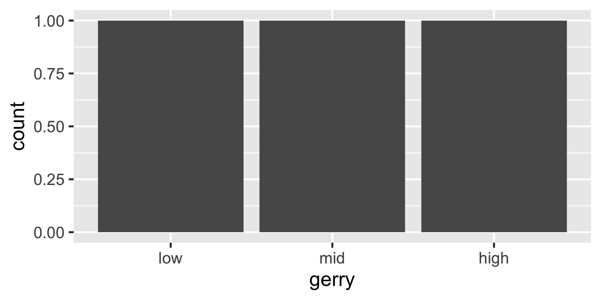

Another glimpse at `gerrymander`

glimpse(gerrymander)

Rows: 435
Columns: 12
$ district   <chr> "AK-AL", "AL-01", "AL-02", "AL-03", "AL-04", "AL-…
$ last_name  <chr> "Young", "Byrne", "Roby", "Rogers", "Aderholt", "…
$ first_name <chr> "Don", "Bradley", "Martha", "Mike D.", "Rob", "Mo…
$ party16    <chr> "R", "R", "R", "R", "R", "R", "R", "D", "R", "R",…
$ clinton16  <dbl> 37.6, 34.1, 33.0, 32.3, 17.4, 31.3, 26.1, 69.8, 3…
$ trump16    <dbl> 52.8, 63.5, 64.9, 65.3, 80.4, 64.7, 70.8, 28.6, 6…
$ dem16      <dbl> 0, 0, 0, 0, 0, 0, 0, 1, 0, 0, 0, 0, 1, 0, 1, 0, 0…
$ state      <chr> "AK", "AL", "AL", "AL", "AL", "AL", "AL", "AL", "…
$ party18    <chr> "R", "R", "R", "R", "R", "R", "R", "D", "R", "R",…
$ dem18      <dbl> 0, 0, 0, 0, 0, 0, 0, 1, 0, 0, 0, 0, 1, 1, 1, 0, 0…
$ flip18     <dbl> 0, 0, 0, 0, 0, 0, 0, 0, 0, 0, 0, 0, 0, 1, 0, 0, 0…
$ gerry      <fct> mid, high, high, high, high, high, high, high, mi…

`mutate()`

We want to use flip18 as a categorical variable
But it’s stored as a numeric
So we need to change its type first, before we can use it as a categorical variable
The mutate() function transforms (mutates) a data frame by creating a new column or updating an existing one

`mutate()` in action

gerrymander |>
  mutate(flip18 = as.factor(flip18))

# A tibble: 435 × 12
   district last_name first_name party16 clinton16 trump16 dem16 state
   <chr>    <chr>     <chr>      <chr>       <dbl>   <dbl> <dbl> <chr>
 1 AK-AL    Young     Don        R            37.6    52.8     0 AK   
 2 AL-01    Byrne     Bradley    R            34.1    63.5     0 AL   
 3 AL-02    Roby      Martha     R            33      64.9     0 AL   
 4 AL-03    Rogers    Mike D.    R            32.3    65.3     0 AL   
 5 AL-04    Aderholt  Rob        R            17.4    80.4     0 AL   
 6 AL-05    Brooks    Mo         R            31.3    64.7     0 AL   
 7 AL-06    Palmer    Gary       R            26.1    70.8     0 AL   
 8 AL-07    Sewell    Terri      D            69.8    28.6     1 AL   
 9 AR-01    Crawford  Rick       R            30.2    65       0 AR   
10 AR-02    Hill      French     R            41.7    52.4     0 AR   
# ℹ 425 more rows
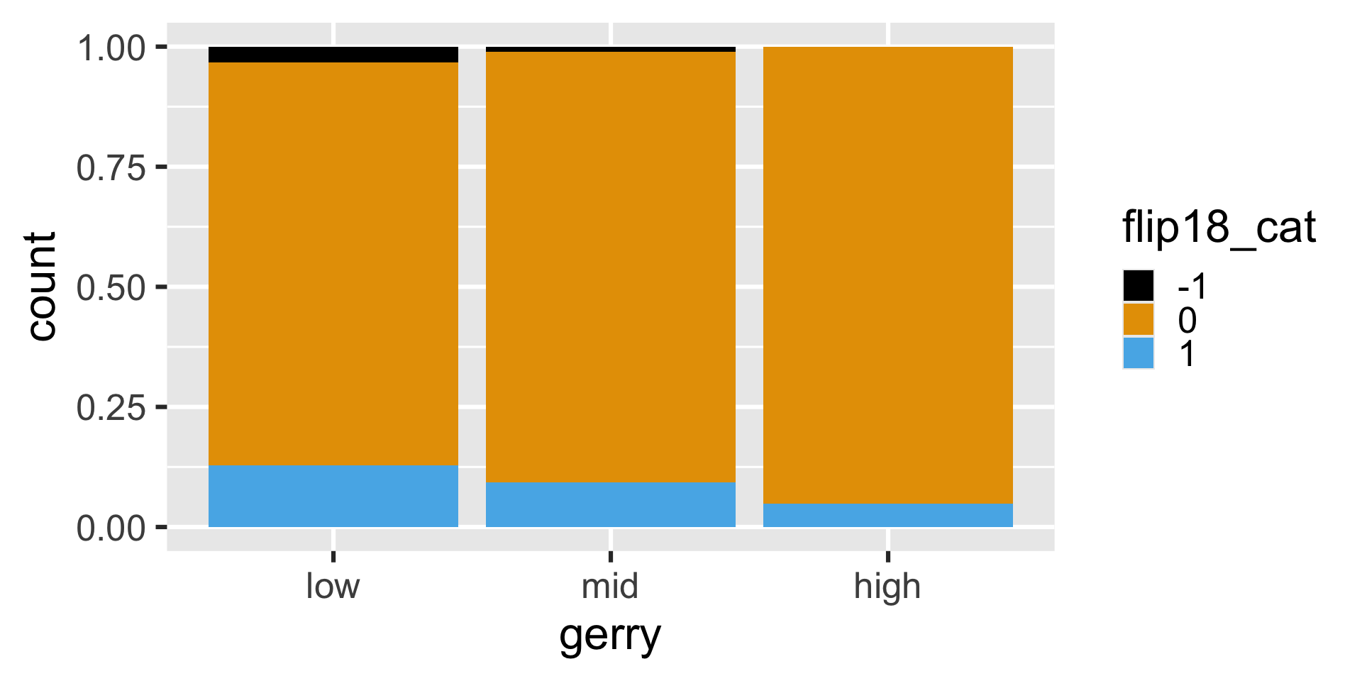
# ℹ 4 more variables: party18 <chr>, dem18 <dbl>, flip18 <fct>,
#   gerry <fct>

Revisit the plot

Is a Congressional District more likely to be flipped to a Democratic seat if it has high prevalence of gerrymandering or low prevalence of gerrymandering?

gerrymander |>
  mutate(flip18 = as.factor(flip18)) |>
  ggplot(aes(x = gerry, fill = flip18)) +
  geom_bar(position = "fill")

Application exercise

ae-04-gerrymander-explore-II

Go to your ae project in RStudio.
If you haven’t yet done so, make sure all of your changes up to this point are committed and pushed, i.e., there’s nothing left in your Git pane.
If you haven’t yet done so, click Pull to get today’s application exercise file: ae-04-gerrymander-explore-II.qmd.
Work through the application exercise in class, and render, commit, and push your edits by the end of class.

Recap: aesthetic mappings

Local aesthetic mappings for a given geom
Global aesthetic mappings for all geoms

Warm-up

While you wait: Participate 📱💻

Reminder: Code style and readability

gerrymander

Packages

From the AE

group_by(), summarize(), count()

What does group_by() do?

Let’s simplify!

group_by()

group_by() |> summarize()

group_by() |> summarize()

summarize()

Spot the difference

count()

count() and sort

mutate()

Flip the question

Flipping vs. gerrymandering prevalence

Another glimpse at gerrymander

mutate()

mutate() in action

Revisit the plot

Application exercise

ae-04-gerrymander-explore-II

Recap: aesthetic mappings

`gerrymander`

`group_by()`, `summarize()`, `count()`

What does `group_by()` do?

`group_by()`

`group_by() |> summarize()`

`group_by() |> summarize()`

`summarize()`

`count()`

`count()` and `sort`

`mutate()`

Another glimpse at `gerrymander`

`mutate()`

`mutate()` in action