x |>
  filter(x1 == "a") |>
select(x1, x2, x5)Exploratory data analysis I
Lecture 5
Warm-up
While you wait: Participate 📱💻
Suppose you have a dataset df with 100 rows and 5 columns: x1, x2, x3, x4, and x5. x1 is a categorical variable with levels a and b. You run the following code:
The resulting data frame will have:
- 3 columns, 50 rows
- 3 columns, 100 rows
- 3 columns, can’t tell how many rows
- 5 columns, 100 rows
- 5 columns, can’t tell how many rows

Scan the QR code or go to app.wooclap.com/sta199. Log in with your Duke NetID.
Announcements
Labs:
Submit PDF on Gradescope by the end of lab session
Make regular commits and push
.qmdand PDF to GitHubGraded primarily for attendance, participation, collaboration, and effort primarily
Feedback provided for correctness
Announcements
Homework: HW 1 due Sunday 11:59pm
- Part 1: Feedback from AI
- No Gradescope submission necessary
- Make regular commits and push
.qmdand PDF to GitHub - Immediate feedback from AI, no grading
- Important: Don’t forget to set homework and question number in the app when requesting feedback
- Part 2: Feedback from humans
- Submit PDF on Gradescope by the deadline
- Make regular commits and push
.qmdand PDF to GitHub - Graded for correctness, feedback provided within ~week
- Important: Don’t forget to select pages corresponding to each question on Gradescope
Exploratory data analysis
Packages
- For the data: usdata
Data: gerrymander
gerrymander# A tibble: 435 × 12
district last_name first_name party16 clinton16 trump16 dem16 state
<chr> <chr> <chr> <chr> <dbl> <dbl> <dbl> <chr>
1 AK-AL Young Don R 37.6 52.8 0 AK
2 AL-01 Byrne Bradley R 34.1 63.5 0 AL
3 AL-02 Roby Martha R 33 64.9 0 AL
4 AL-03 Rogers Mike D. R 32.3 65.3 0 AL
5 AL-04 Aderholt Rob R 17.4 80.4 0 AL
6 AL-05 Brooks Mo R 31.3 64.7 0 AL
7 AL-06 Palmer Gary R 26.1 70.8 0 AL
8 AL-07 Sewell Terri D 69.8 28.6 1 AL
9 AR-01 Crawford Rick R 30.2 65 0 AR
10 AR-02 Hill French R 41.7 52.4 0 AR
# ℹ 425 more rows
# ℹ 4 more variables: party18 <chr>, dem18 <dbl>, flip18 <dbl>,
# gerry <fct>What is gerrymandering?
Participate 📱💻
You are given a new dataset to analyze. What are some of the first things you would do to get to know the data?
Scan the QR code or go to app.wooclap.com/sta199. Log in with your Duke NetID.
Data: gerrymander
glimpse(gerrymander)Rows: 435
Columns: 12
$ district <chr> "AK-AL", "AL-01", "AL-02", "AL-03", "AL-04", "AL-…
$ last_name <chr> "Young", "Byrne", "Roby", "Rogers", "Aderholt", "…
$ first_name <chr> "Don", "Bradley", "Martha", "Mike D.", "Rob", "Mo…
$ party16 <chr> "R", "R", "R", "R", "R", "R", "R", "D", "R", "R",…
$ clinton16 <dbl> 37.6, 34.1, 33.0, 32.3, 17.4, 31.3, 26.1, 69.8, 3…
$ trump16 <dbl> 52.8, 63.5, 64.9, 65.3, 80.4, 64.7, 70.8, 28.6, 6…
$ dem16 <dbl> 0, 0, 0, 0, 0, 0, 0, 1, 0, 0, 0, 0, 1, 0, 1, 0, 0…
$ state <chr> "AK", "AL", "AL", "AL", "AL", "AL", "AL", "AL", "…
$ party18 <chr> "R", "R", "R", "R", "R", "R", "R", "D", "R", "R",…
$ dem18 <dbl> 0, 0, 0, 0, 0, 0, 0, 1, 0, 0, 0, 0, 1, 1, 1, 0, 0…
$ flip18 <dbl> 0, 0, 0, 0, 0, 0, 0, 0, 0, 0, 0, 0, 0, 1, 0, 0, 0…
$ gerry <fct> mid, high, high, high, high, high, high, high, mi…Data: gerrymander
Rows: Congressional districts
-
Columns:
Congressional district and state
2016 election: winning party, % for Clinton, % for Trump, whether a Democrat won the House election, name of election winner
2018 election: winning party, whether a Democrat won the 2018 House election
Whether a Democrat flipped the seat in the 2018 election
Prevalence of gerrymandering: low, mid, and high
Variable types: district
| Variable | Type |
|---|---|
district |
categorical, ID |
last_name |
|
first_name |
|
party16 |
|
clinton16 |
|
trump16 |
|
dem16 |
|
state |
|
party18 |
|
dem18 |
|
flip18 |
|
gerry |
gerrymander |>
  select(district)
# A tibble: 435 × 1
district
<chr>
1 AK-AL
2 AL-01
3 AL-02
4 AL-03
5 AL-04
6 AL-05
7 AL-06
8 AL-07
9 AR-01
10 AR-02
# ℹ 425 more rowsVariable types: last_name
| Variable | Type |
|---|---|
district |
categorical, ID |
last_name |
categorical, ID |
first_name |
|
party16 |
|
clinton16 |
|
trump16 |
|
dem16 |
|
state |
|
party18 |
|
dem18 |
|
flip18 |
|
gerry |
gerrymander |>
  select(last_name)
# A tibble: 435 × 1
last_name
<chr>
1 Young
2 Byrne
3 Roby
4 Rogers
5 Aderholt
6 Brooks
7 Palmer
8 Sewell
9 Crawford
10 Hill
# ℹ 425 more rowsVariable types: first_name
| Variable | Type |
|---|---|
district |
categorical, ID |
last_name |
categorical, ID |
first_name |
categorical, ID |
party16 |
|
clinton16 |
|
trump16 |
|
dem16 |
|
state |
|
party18 |
|
dem18 |
|
flip18 |
|
gerry |
gerrymander |>
  select(first_name)
# A tibble: 435 × 1
first_name
<chr>
1 Don
2 Bradley
3 Martha
4 Mike D.
5 Rob
6 Mo
7 Gary
8 Terri
9 Rick
10 French
# ℹ 425 more rowsVariable types: party16
| Variable | Type |
|---|---|
district |
categorical, ID |
last_name |
categorical, ID |
first_name |
categorical, ID |
party16 |
categorical |
clinton16 |
|
trump16 |
|
dem16 |
|
state |
|
party18 |
|
dem18 |
|
flip18 |
|
gerry |
gerrymander |>
  select(party16)
# A tibble: 435 × 1
party16
<chr>
1 R
2 R
3 R
4 R
5 R
6 R
7 R
8 D
9 R
10 R
# ℹ 425 more rowsVariable types: clinton16
| Variable | Type |
|---|---|
district |
categorical, ID |
last_name |
categorical, ID |
first_name |
categorical, ID |
party16 |
categorical |
clinton16 |
numerical, continuous |
trump16 |
|
dem16 |
|
state |
|
party18 |
|
dem18 |
|
flip18 |
|
gerry |
gerrymander |>
  select(clinton16)
# A tibble: 435 × 1
clinton16
<dbl>
1 37.6
2 34.1
3 33
4 32.3
5 17.4
6 31.3
7 26.1
8 69.8
9 30.2
10 41.7
# ℹ 425 more rowsVariable types: trump16
| Variable | Type |
|---|---|
district |
categorical, ID |
last_name |
categorical, ID |
first_name |
categorical, ID |
party16 |
categorical |
clinton16 |
numerical, continuous |
trump16 |
numerical, continuous |
dem16 |
|
state |
|
party18 |
|
dem18 |
|
flip18 |
|
gerry |
gerrymander |>
  select(trump16)
# A tibble: 435 × 1
trump16
<dbl>
1 52.8
2 63.5
3 64.9
4 65.3
5 80.4
6 64.7
7 70.8
8 28.6
9 65
10 52.4
# ℹ 425 more rowsVariable types: dem16
| Variable | Type |
|---|---|
district |
categorical, ID |
last_name |
categorical, ID |
first_name |
categorical, ID |
party16 |
categorical |
clinton16 |
numerical, continuous |
trump16 |
numerical, continuous |
dem16 |
categorical |
state |
|
party18 |
|
dem18 |
|
flip18 |
|
gerry |
gerrymander |>
  select(dem16)
# A tibble: 435 × 1
dem16
<dbl>
1 0
2 0
3 0
4 0
5 0
6 0
7 0
8 1
9 0
10 0
# ℹ 425 more rowsVariable types: state
| Variable | Type |
|---|---|
district |
categorical, ID |
last_name |
categorical, ID |
first_name |
categorical, ID |
party16 |
categorical |
clinton16 |
numerical, continuous |
trump16 |
numerical, continuous |
dem16 |
categorical |
state |
categorical |
party18 |
|
dem18 |
|
flip18 |
|
gerry |
gerrymander |>
  select(state)
# A tibble: 435 × 1
state
<chr>
1 AK
2 AL
3 AL
4 AL
5 AL
6 AL
7 AL
8 AL
9 AR
10 AR
# ℹ 425 more rowsVariable types: party18
| Variable | Type |
|---|---|
district |
categorical, ID |
last_name |
categorical, ID |
first_name |
categorical, ID |
party16 |
categorical |
clinton16 |
numerical, continuous |
trump16 |
numerical, continuous |
dem16 |
categorical |
state |
categorical |
party18 |
categorical |
dem18 |
|
flip18 |
|
gerry |
gerrymander |>
  select(party18)
# A tibble: 435 × 1
party18
<chr>
1 R
2 R
3 R
4 R
5 R
6 R
7 R
8 D
9 R
10 R
# ℹ 425 more rowsVariable types: dem18
| Variable | Type |
|---|---|
district |
categorical, ID |
last_name |
categorical, ID |
first_name |
categorical, ID |
party16 |
categorical |
clinton16 |
numerical, continuous |
trump16 |
numerical, continuous |
dem16 |
categorical |
state |
categorical |
party18 |
categorical |
dem18 |
categorical |
flip18 |
|
gerry |
gerrymander |>
  select(dem18)
# A tibble: 435 × 1
dem18
<dbl>
1 0
2 0
3 0
4 0
5 0
6 0
7 0
8 1
9 0
10 0
# ℹ 425 more rowsVariable types: flip18
| Variable | Type |
|---|---|
district |
categorical, ID |
last_name |
categorical, ID |
first_name |
categorical, ID |
party16 |
categorical |
clinton16 |
numerical, continuous |
trump16 |
numerical, continuous |
dem16 |
categorical |
state |
categorical |
party18 |
categorical |
dem18 |
categorical |
flip18 |
categorical |
gerry |
gerrymander |>
  select(flip18)
# A tibble: 435 × 1
flip18
<dbl>
1 0
2 0
3 0
4 0
5 0
6 0
7 0
8 0
9 0
10 0
# ℹ 425 more rowsVariable types: gerry
| Variable | Type |
|---|---|
district |
categorical, ID |
last_name |
categorical, ID |
first_name |
categorical, ID |
party16 |
categorical |
clinton16 |
numerical, continuous |
trump16 |
numerical, continuous |
dem16 |
categorical |
state |
categorical |
party18 |
categorical |
dem18 |
categorical |
flip18 |
categorical |
gerry |
categorical, ordinal |
gerrymander |>
  select(gerry)
# A tibble: 435 × 1
gerry
<fct>
1 mid
2 high
3 high
4 high
5 high
6 high
7 high
8 high
9 mid
10 mid
# ℹ 425 more rowsUnivariate analysis
Univariate analysis
Analyzing a single variable:
Numerical: histogram, box plot, density plot, etc.
Categorical: bar plot, pie chart, etc.
Histogram - Step 1
ggplot(gerrymander)
Histogram - Step 2

Histogram - Step 3
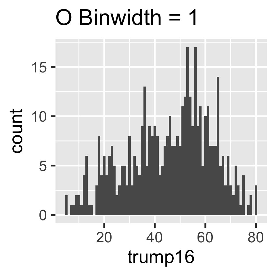
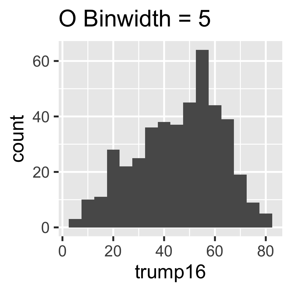
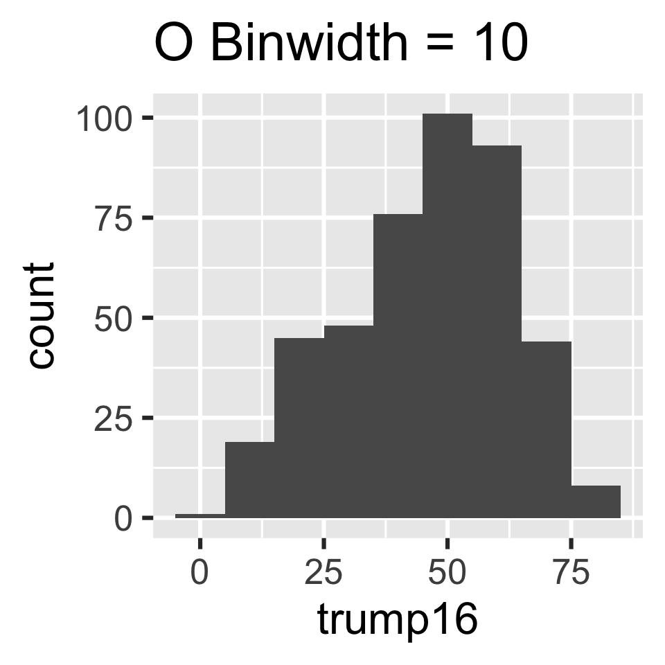
Participate 📱💻
Which of the following histograms has the most appropriate binwidth for visualizing the distribution of trump16?
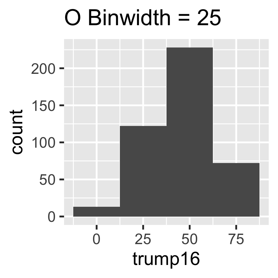
Scan the QR code or go to app.wooclap.com/sta199. Log in with your Duke NetID.
Histogram - Step 4

Histogram - Step 5
Box plot - Step 1
ggplot(gerrymander)
Box plot - Step 2

Box plot - Step 3
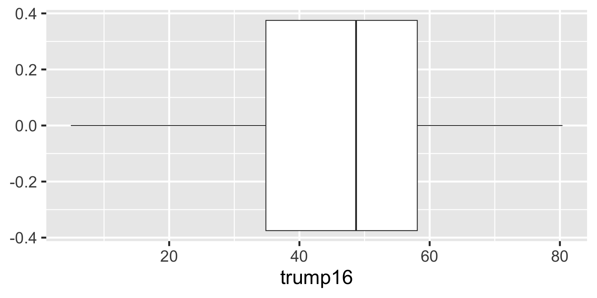
Box plot - Alternative Step 2 + 3
ggplot(gerrymander, aes(y = trump16)) +
  geom_boxplot()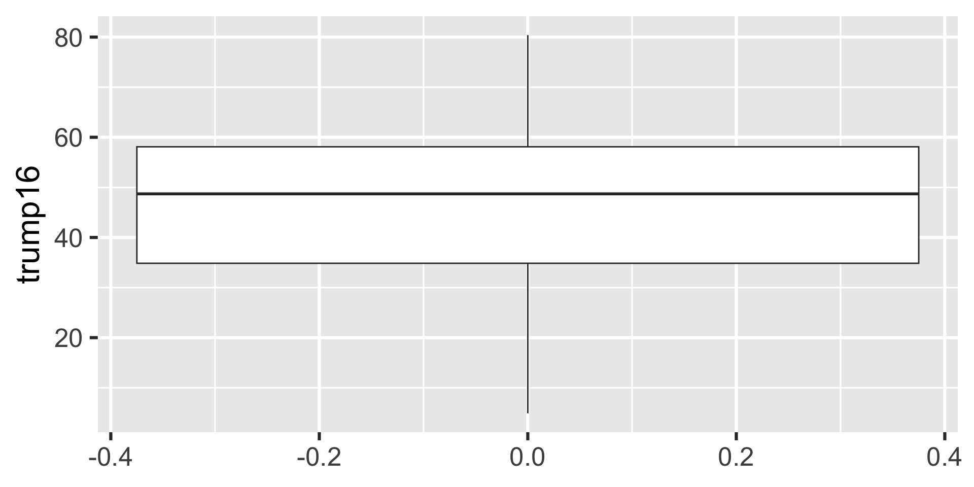
Box plot - Step 4
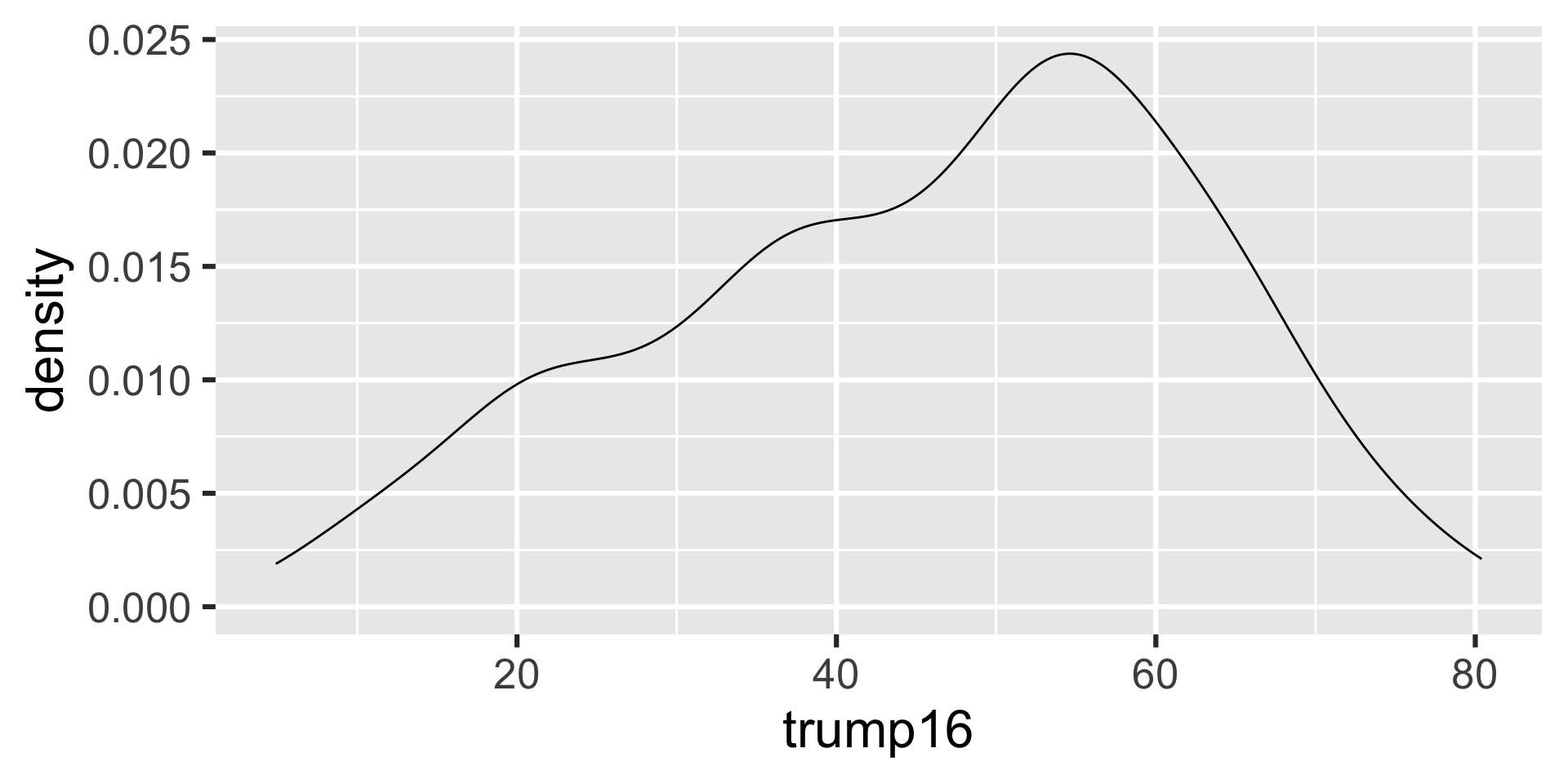
Density plot - Step 1
ggplot(gerrymander)
Density plot - Step 2
Density plot - Step 3
Density plot - Step 4
ggplot(gerrymander, aes(x = trump16)) +
  geom_density(color = "firebrick")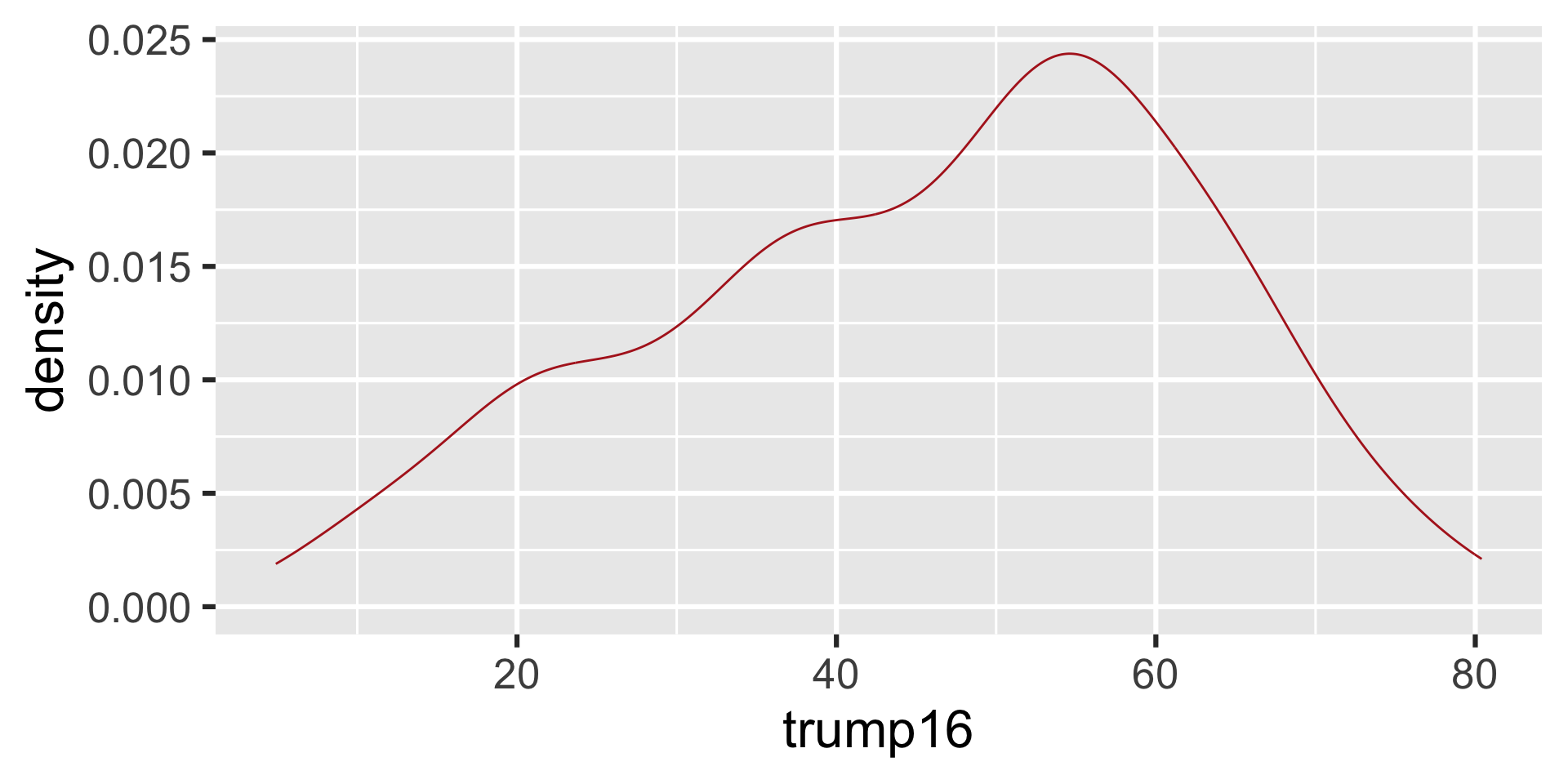
Density plot - Step 5
ggplot(gerrymander, aes(x = trump16)) +
  geom_density(color = "firebrick", fill = "firebrick1")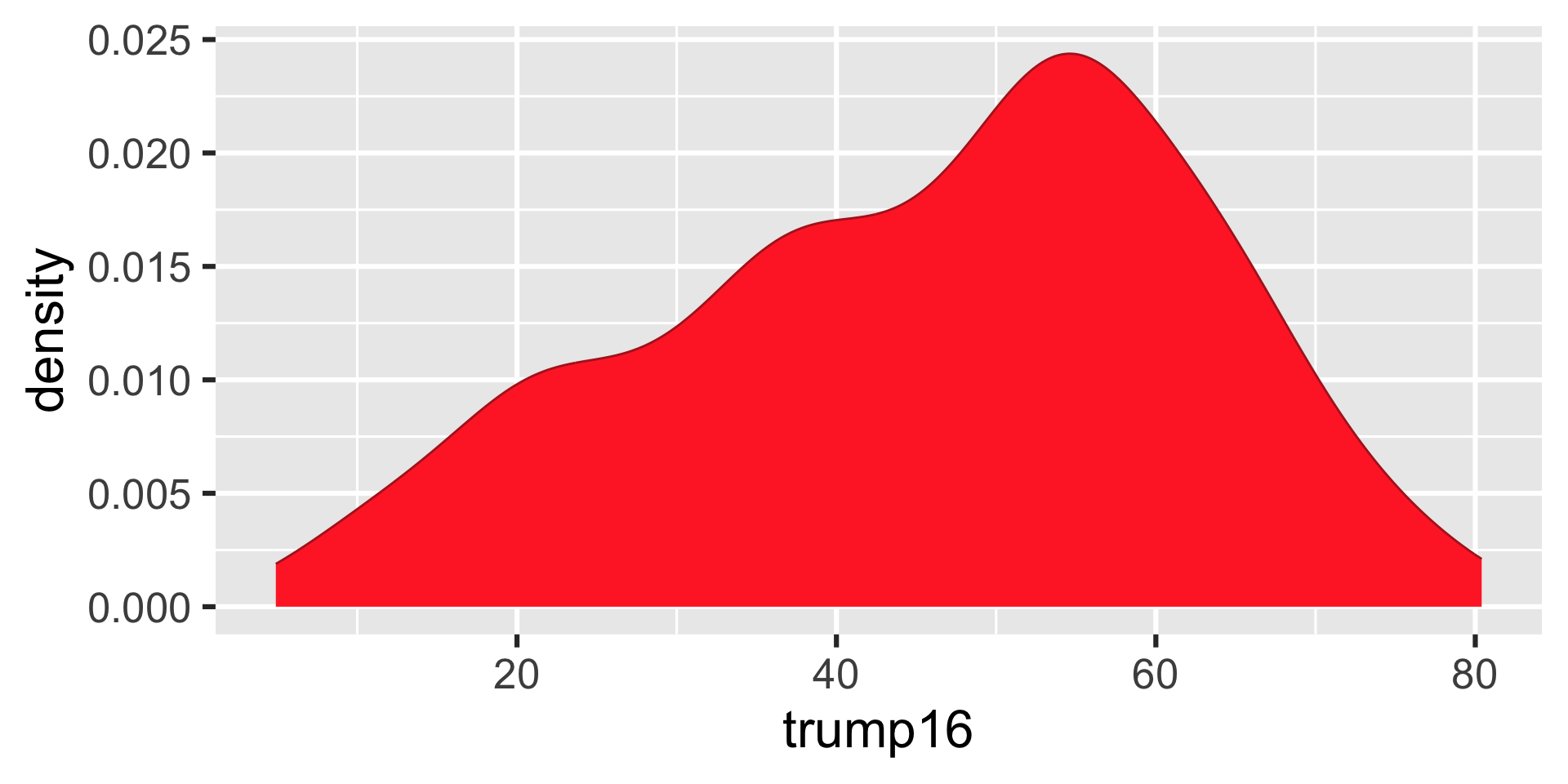
Density plot - Step 6
ggplot(gerrymander, aes(x = trump16)) +
  geom_density(color = "firebrick", fill = "firebrick1", alpha = 0.5)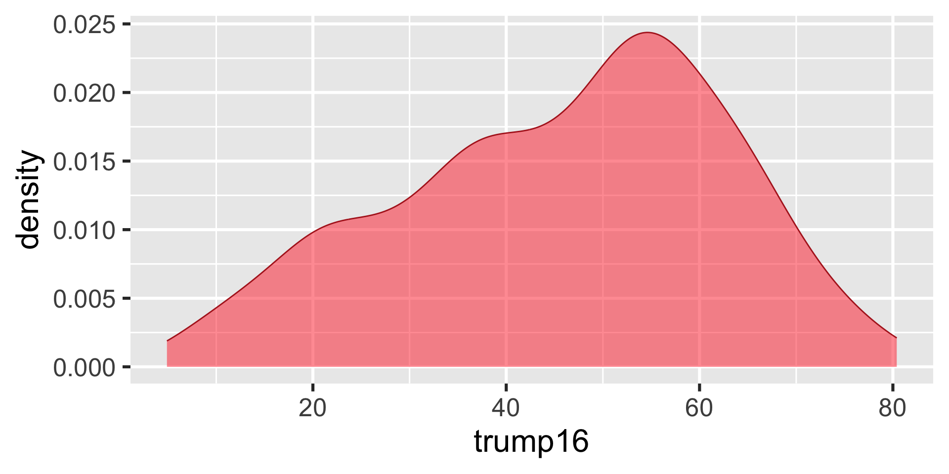
Density plot - Step 7
ggplot(gerrymander, aes(x = trump16)) +
  geom_density(color = "firebrick", fill = "firebrick1", alpha = 0.5, linewidth = 1)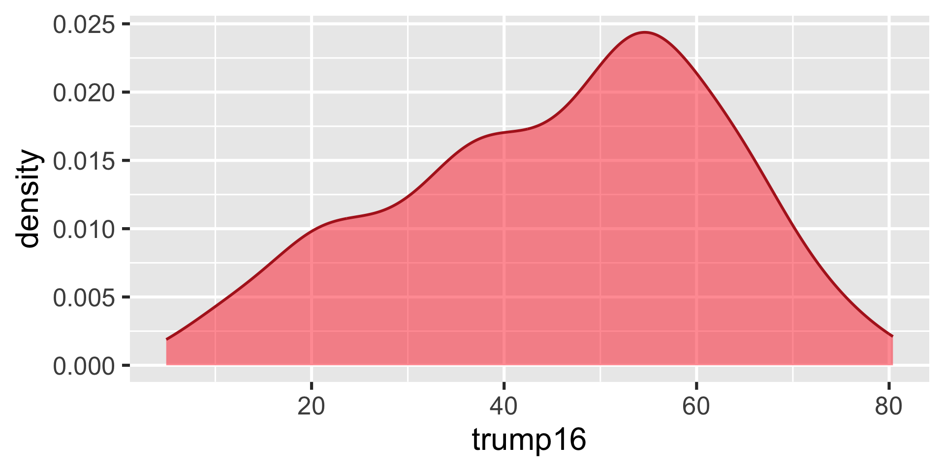
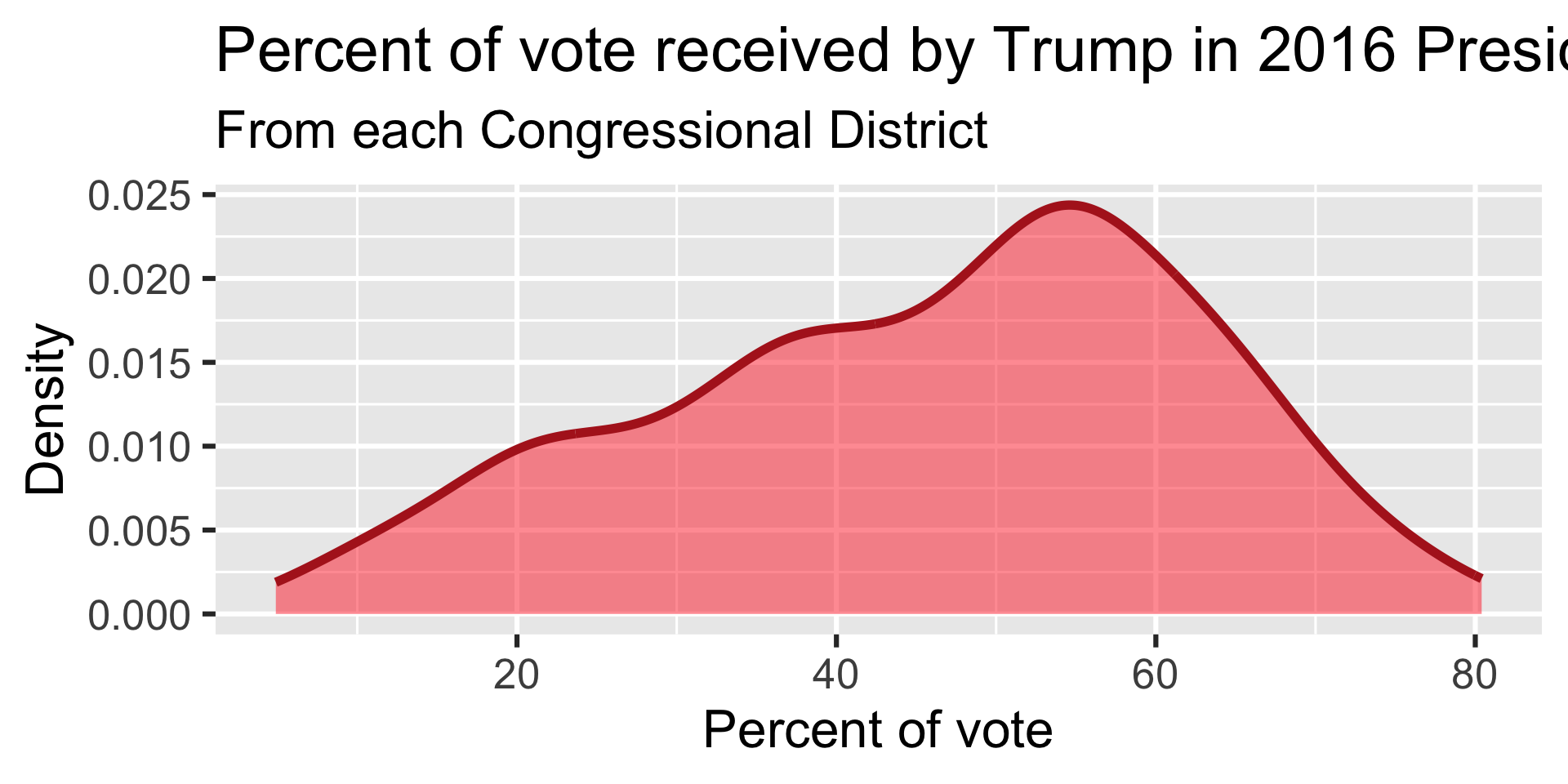
Density plot - Step 8
Summary statistics
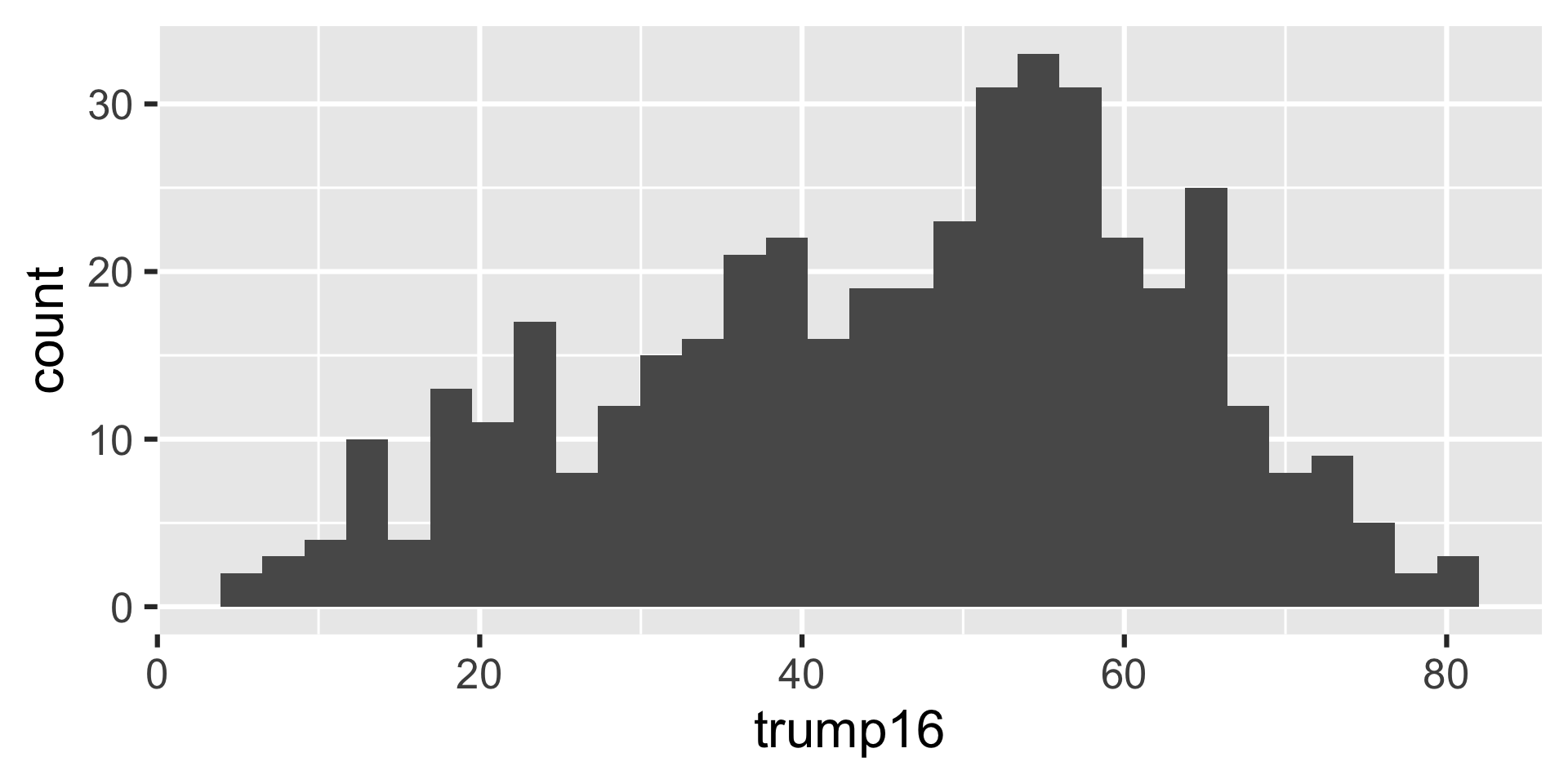
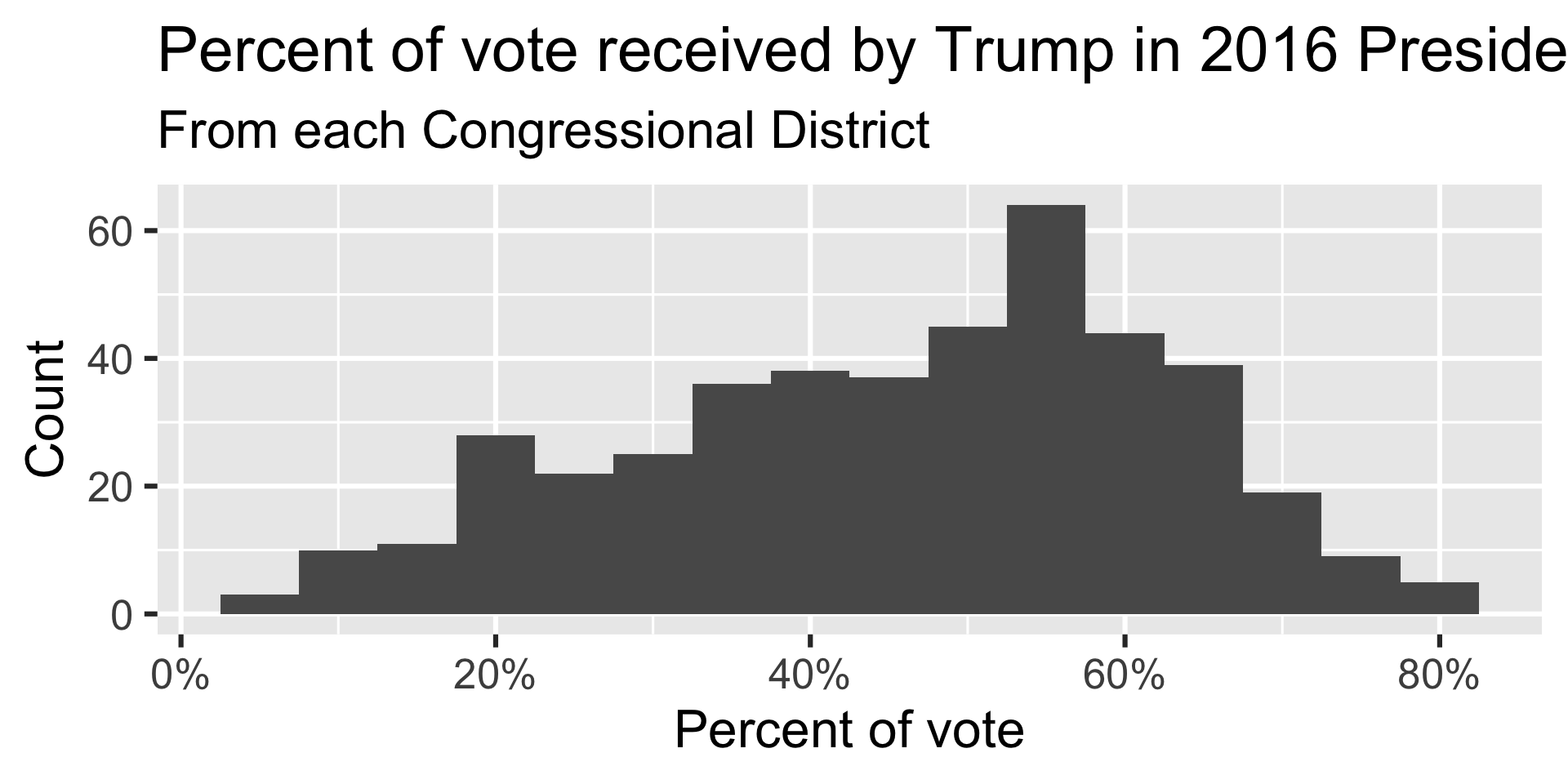
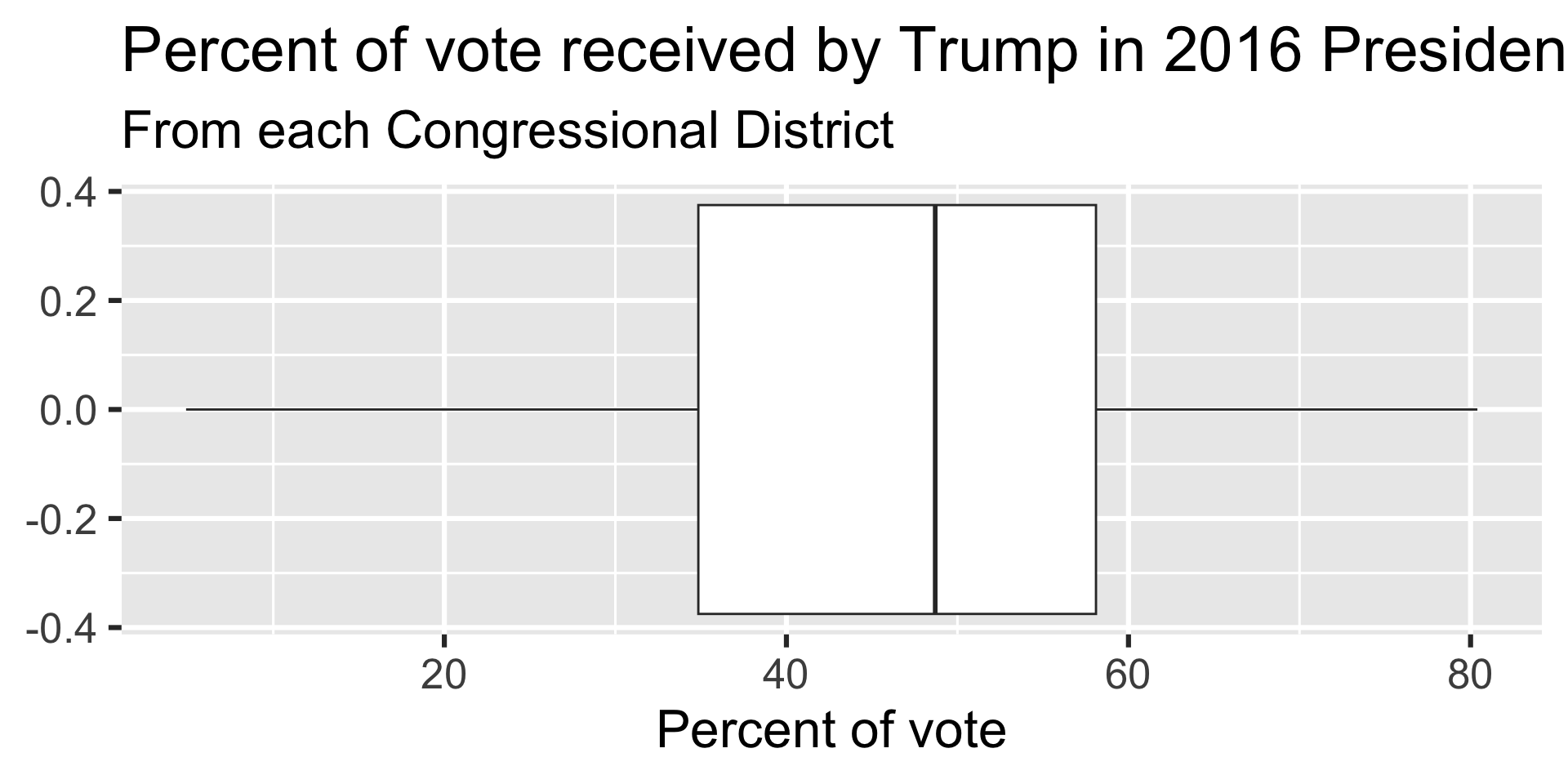
Distribution of votes for Trump in the 2016 election
Describe the distribution of percent of vote received by Trump in 2016 Presidential Election from Congressional Districts.
Shape: The distribution of votes for Trump in the 2016 election from Congressional Districts is unimodal and left-skewed.
Center: The percent of vote received by Trump in the 2016 Presidential Election from a typical Congressional Districts is 48.7%.
Spread: In the middle 50% of Congressional Districts, 34.8% to 58.1% of voters voted for Trump in the 2016 Presidential Election.
Unusual observations: -
Bivariate analysis
Bivariate analysis
Analyzing the relationship between two variables:
Numerical + numerical: scatterplot
Numerical + categorical: side-by-side box plots, violin plots, etc.
Categorical + categorical: stacked bar plots
Using an aesthetic (e.g., fill, color, shape, etc.) or facets to represent the second variable in any plot
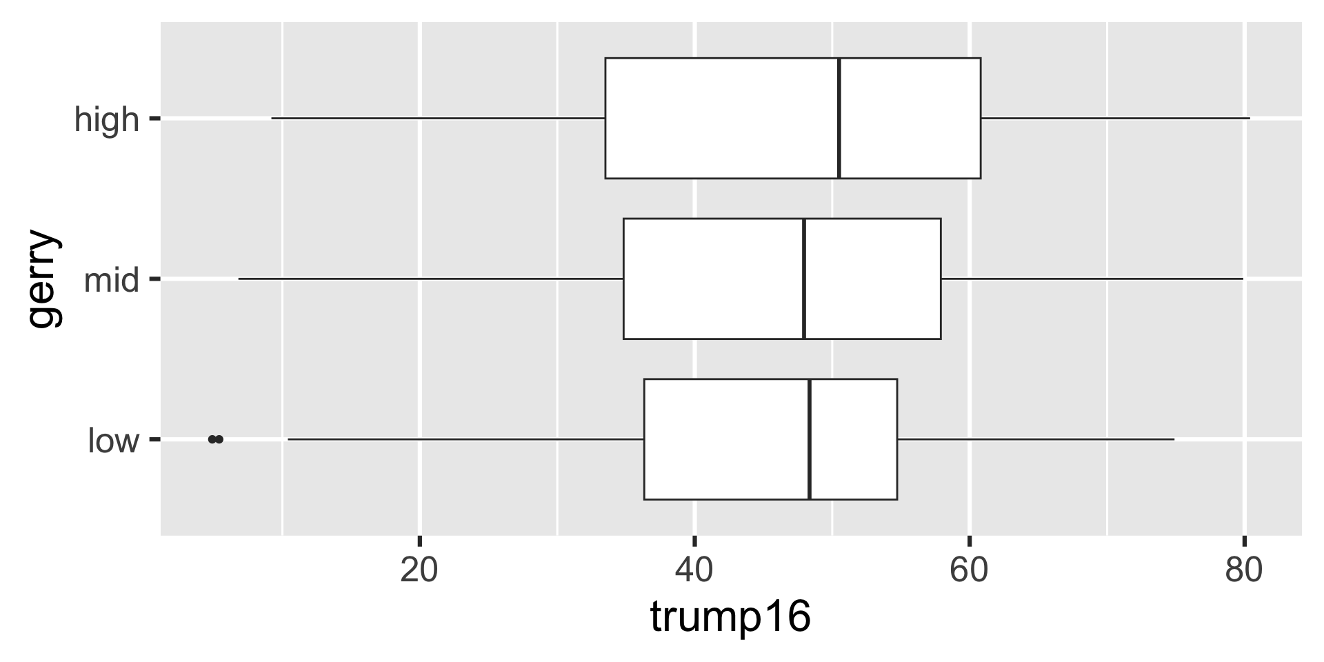
Side-by-side box plots
Summary statistics
Participate 📱💻
What goes in the [blank] in the code below to do the following step for each level of gerry?
Scan the QR code or go to app.wooclap.com/sta199. Log in with your Duke NetID.
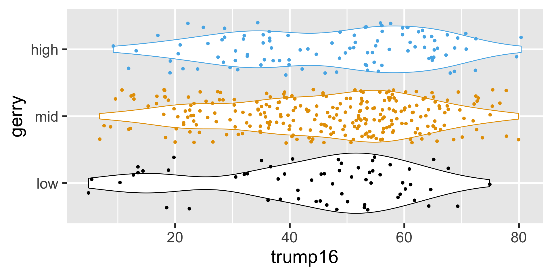
Grouped summary statistics
gerrymander |>
  group_by(gerry) |>
  summarize(
    min = min(trump16),
    q25 = quantile(trump16, 0.25),
    median = median(trump16),
    q75 = quantile(trump16, 0.75),
    max = max(trump16),
  )
# A tibble: 3 × 6
gerry min q25 median q75 max
<fct> <dbl> <dbl> <dbl> <dbl> <dbl>
1 low 4.9 36.3 48.4 54.7 74.9
2 mid 6.8 34.8 48.0 57.9 79.9
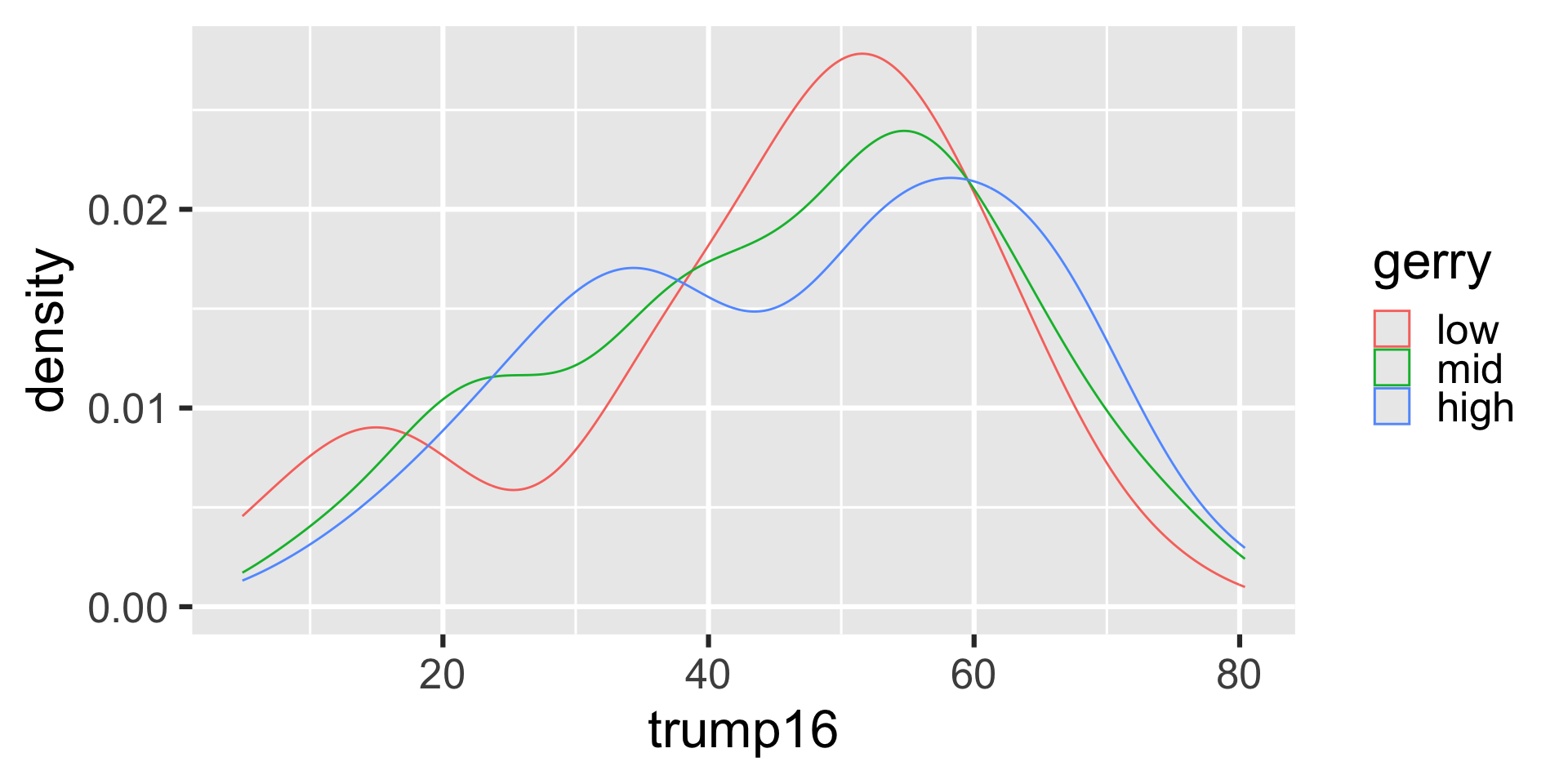
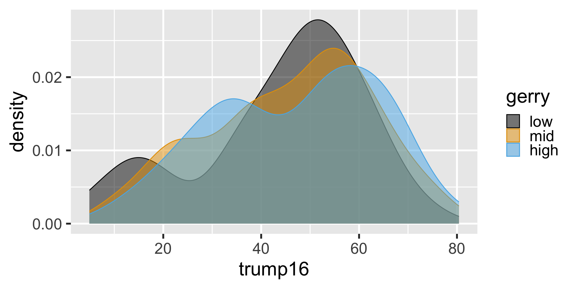
3 high 9.2 33.5 50.5 60.8 80.4Density plots
Filled density plots
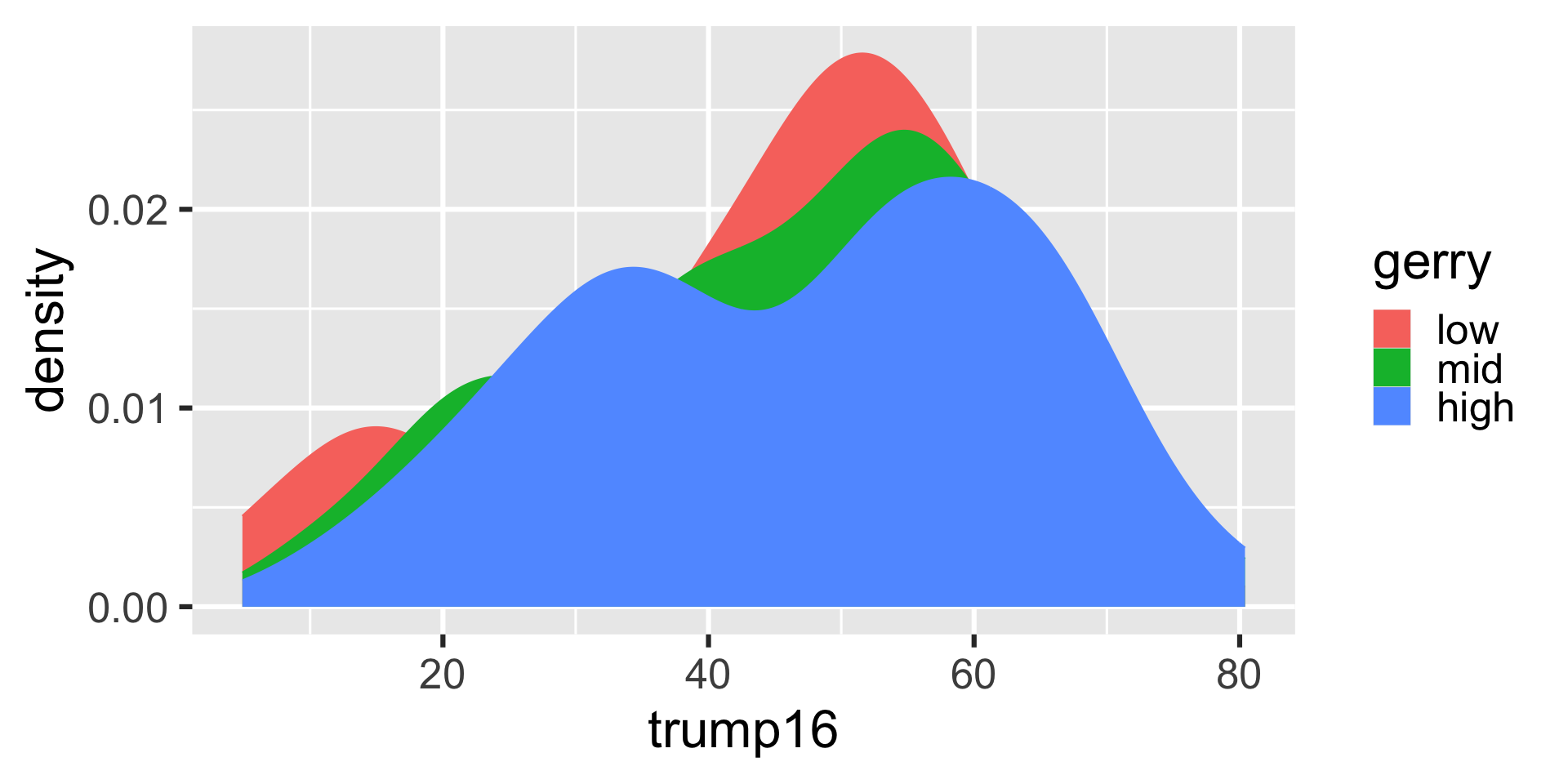
Better filled density plots
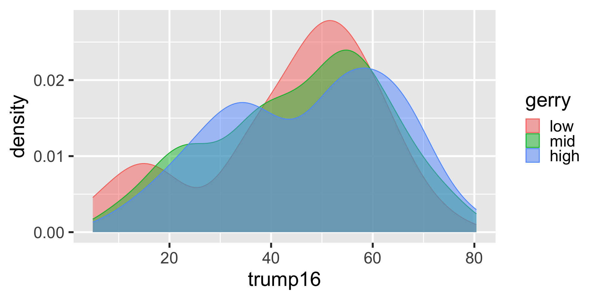
Better colors
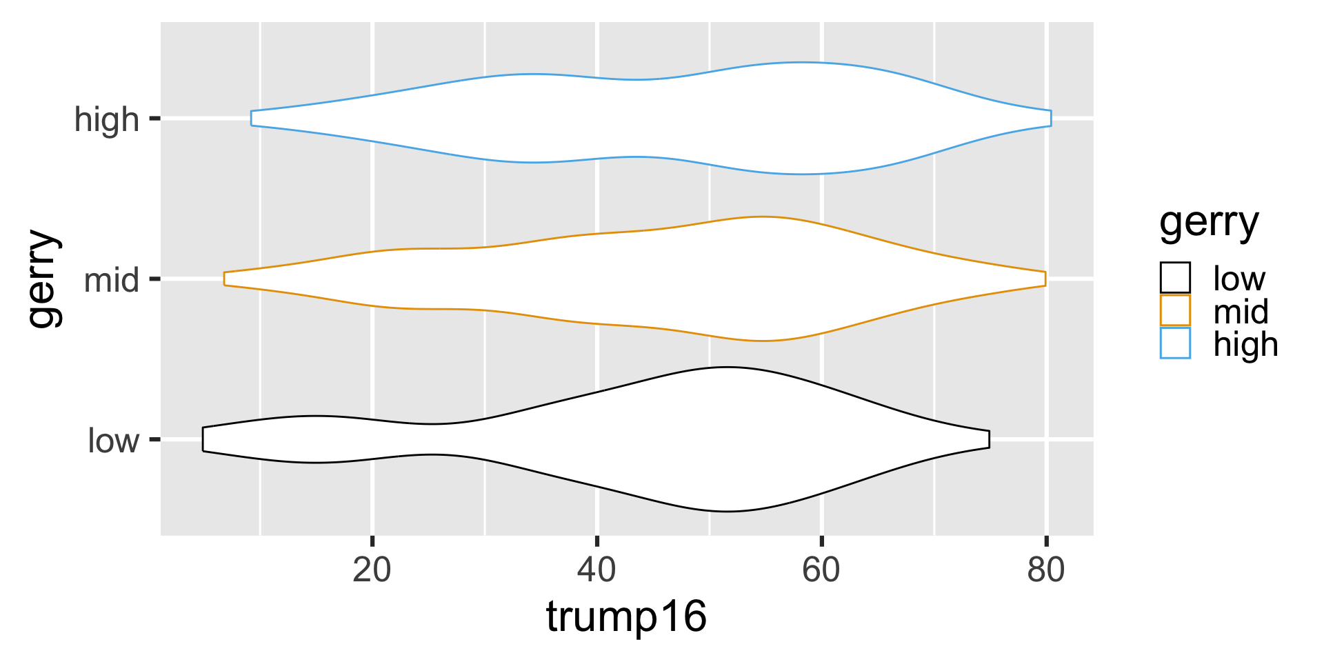
Violin plots
Multiple geoms
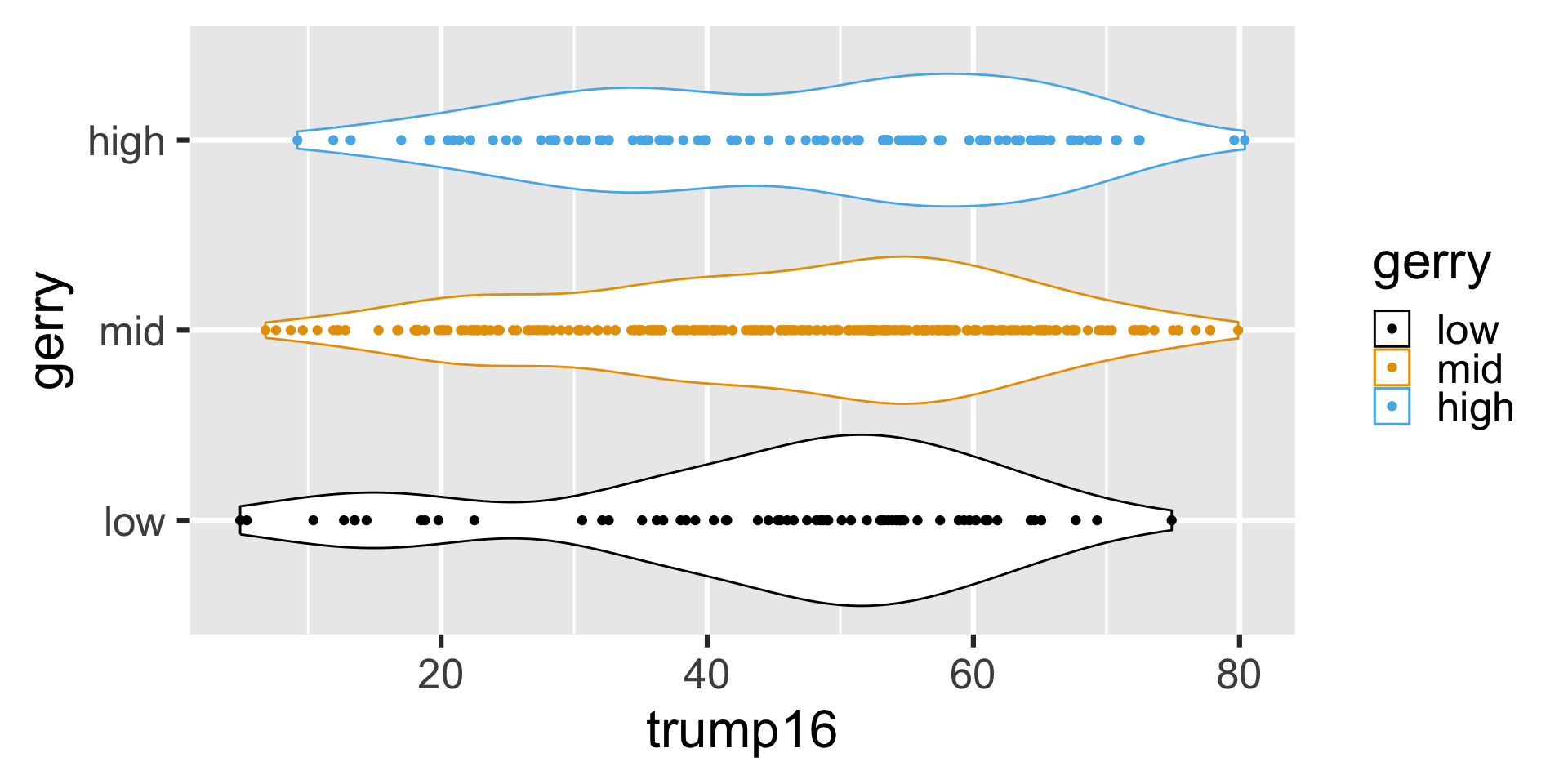
Multiple geoms
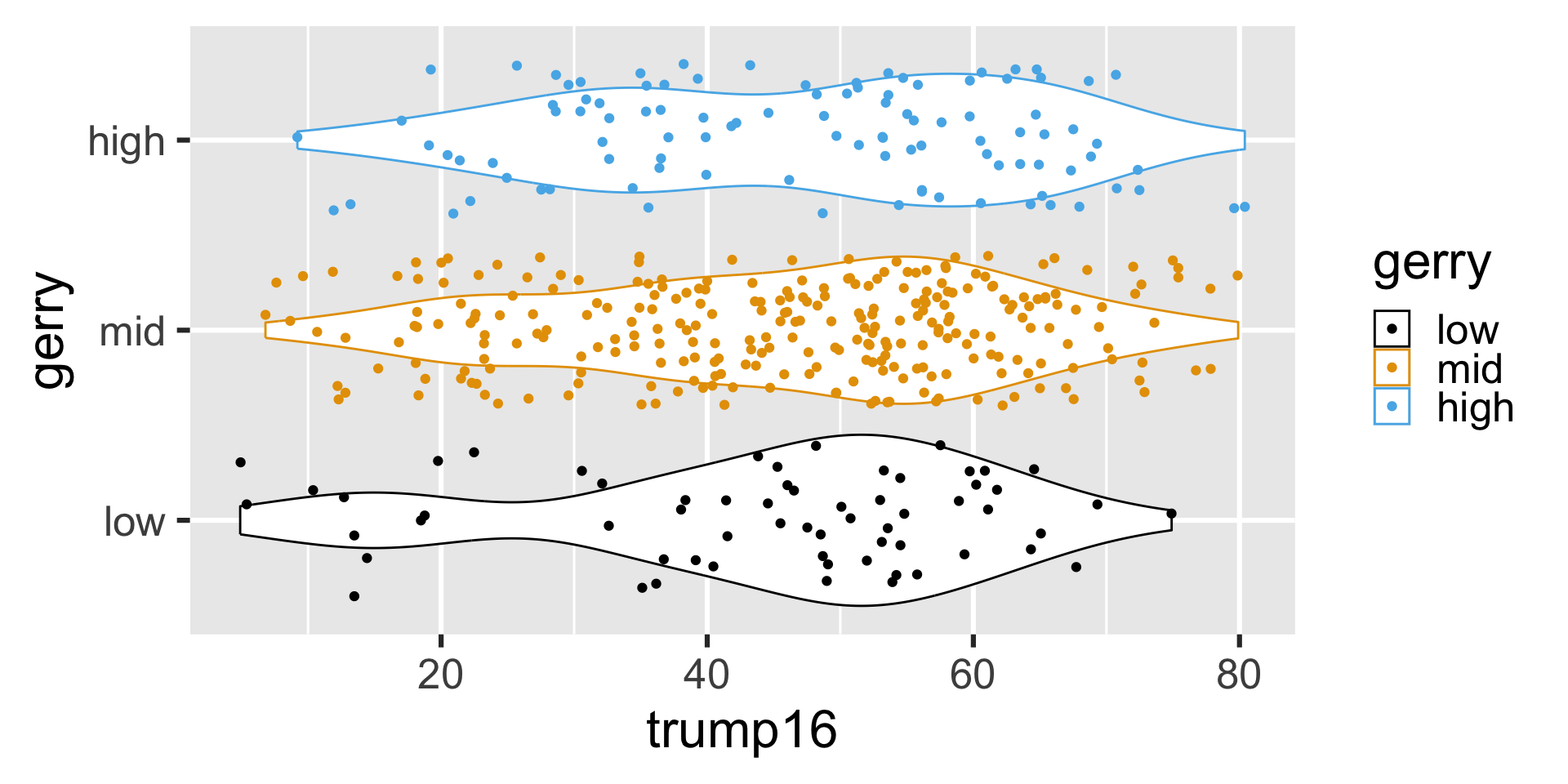
Remove legend
Multivariate analysis
Multivariate analysis
Analyzing the relationship between multiple variables:
In general, one variable is identified as the outcome of interest
The remaining variables are predictors or explanatory variables
-
Plots for exploring multivariate relationships are the same as those for bivariate relationships, but conditional on one or more variables
- Conditioning can be done via faceting or aesthetic mappings (e.g., scatterplot of
yvs.x1, colored byx2, faceted byx3)
- Conditioning can be done via faceting or aesthetic mappings (e.g., scatterplot of
-
Summary statistics for exploring multivariate relationships are the same as those for bivariate relationships, but conditional on one or more variables
- Conditioning can be done via grouping (e.g., correlation between
yandx1, grouped by levels ofx2andx3)
- Conditioning can be done via grouping (e.g., correlation between
Application exercise
ae-03-gerrymander-explore-I
Go to your ae project in RStudio.
If you haven’t yet done so, make sure all of your changes up to this point are committed and pushed, i.e., there’s nothing left in your Git pane.
If you haven’t yet done so, click Pull to get today’s application exercise file: ae-03-gerrymander-explore-I.qmd.
Work through the application exercise in class, and render, commit, and push your edits by the end of class.