Exploratory data analysis I
Lecture 5
September 9, 2025
While you wait: Participate 📱💻
Suppose you have a dataset df with 100 rows and 5 columns: x1, x2, x3, x4, and x5. x1 is a categorical variable with levels a and b. You run the following code:
The resulting data frame will have:
- 3 columns, 50 rows
- 3 columns, 100 rows
- 3 columns, can’t tell how many rows
- 5 columns, 100 rows
- 5 columns, can’t tell how many rows

Scan the QR code or go to app.wooclap.com/sta199. Log in with your Duke NetID.
Participate 📱💻
You are given a new dataset to analyze. What are some of the first things you would do to get to know the data?
Scan the QR code or go to app.wooclap.com/sta199. Log in with your Duke NetID.
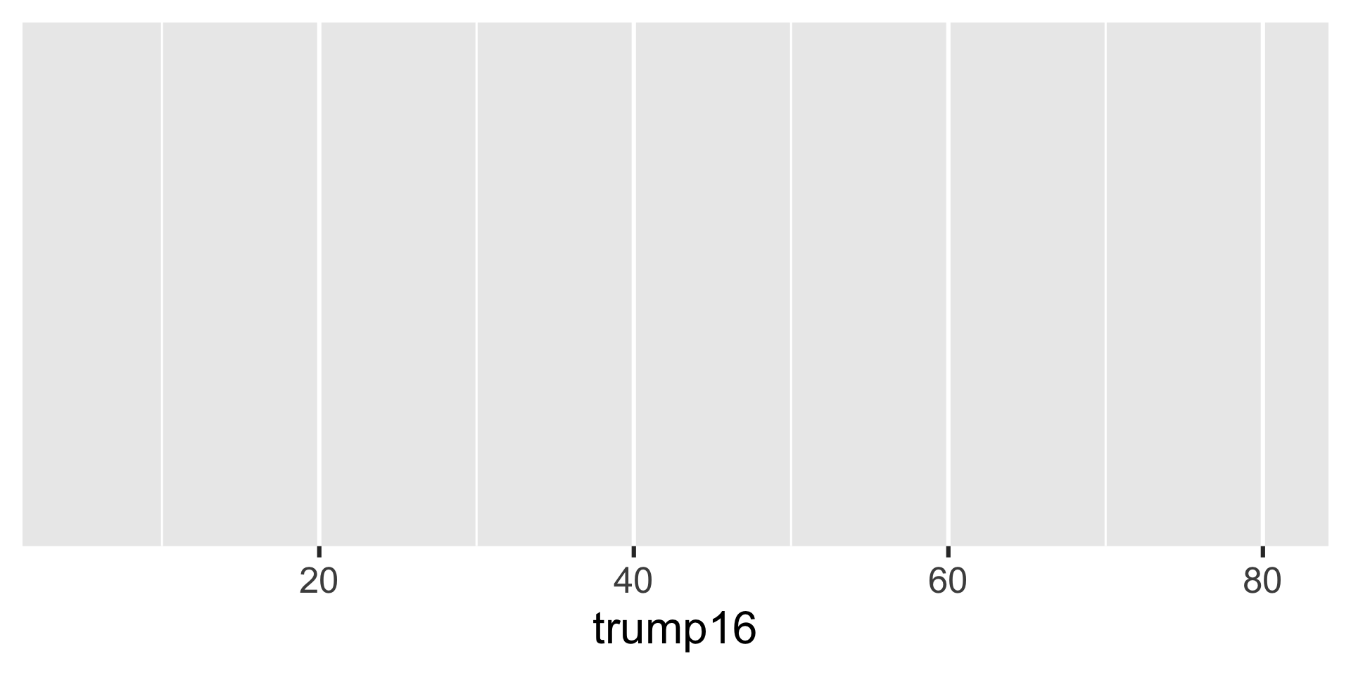
Histogram - Step 1

Histogram - Step 2

Histogram - Step 3
`stat_bin()` using `bins = 30`. Pick better value with `binwidth`.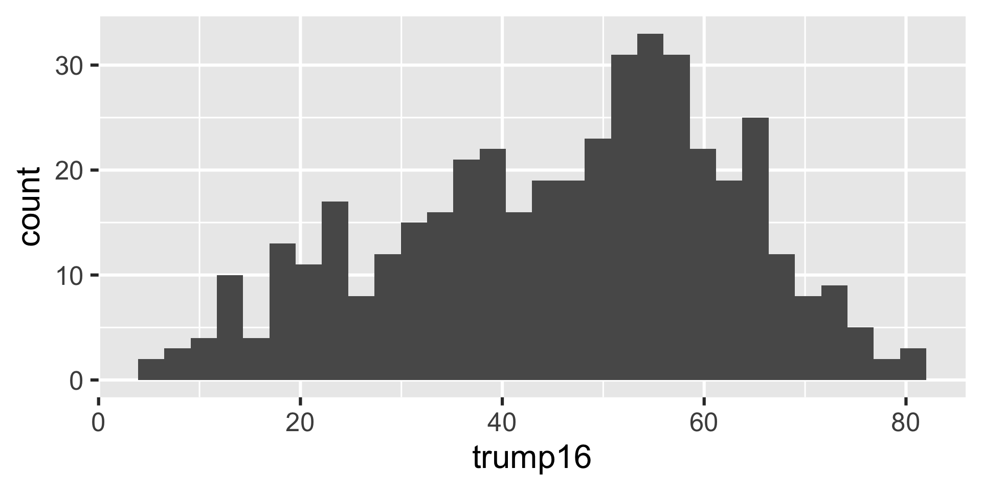
Participate 📱💻
Which of the following histograms has the most appropriate binwidth for visualizing the distribution of trump16?
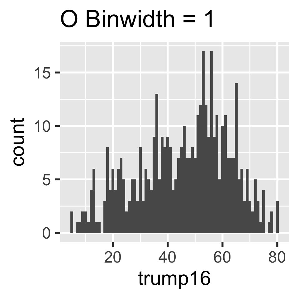
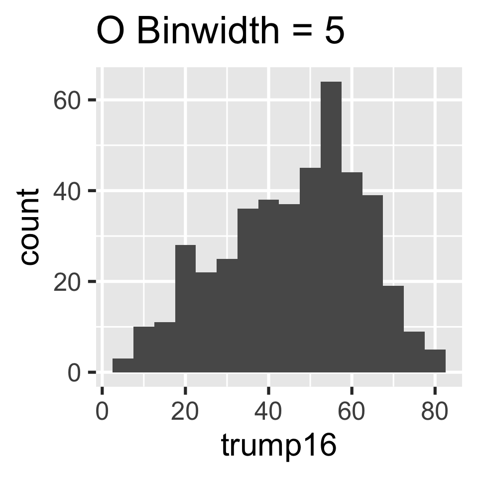
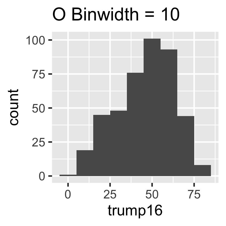
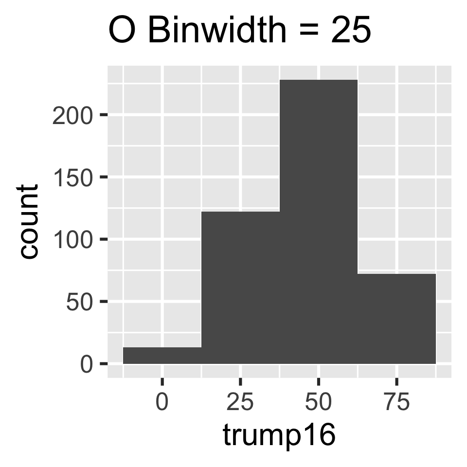
Scan the QR code or go to app.wooclap.com/sta199. Log in with your Duke NetID.
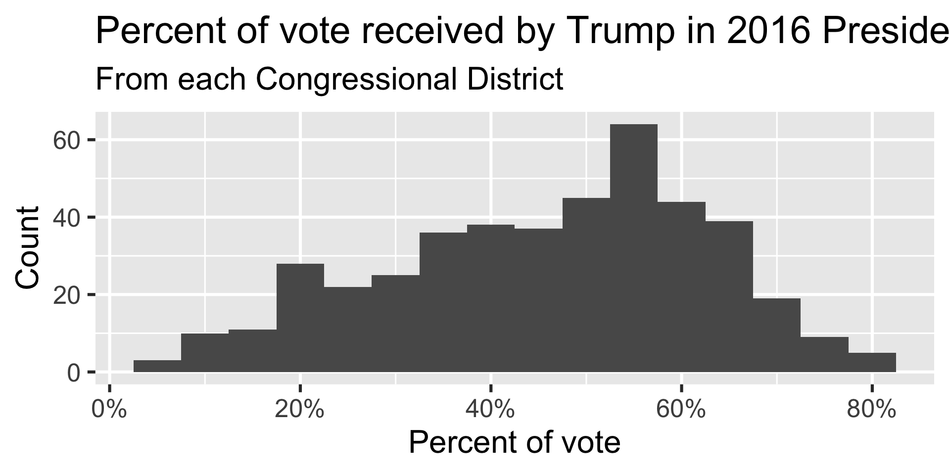
Histogram - Step 4

Histogram - Step 5
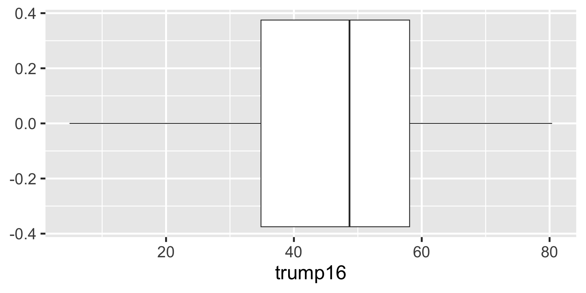
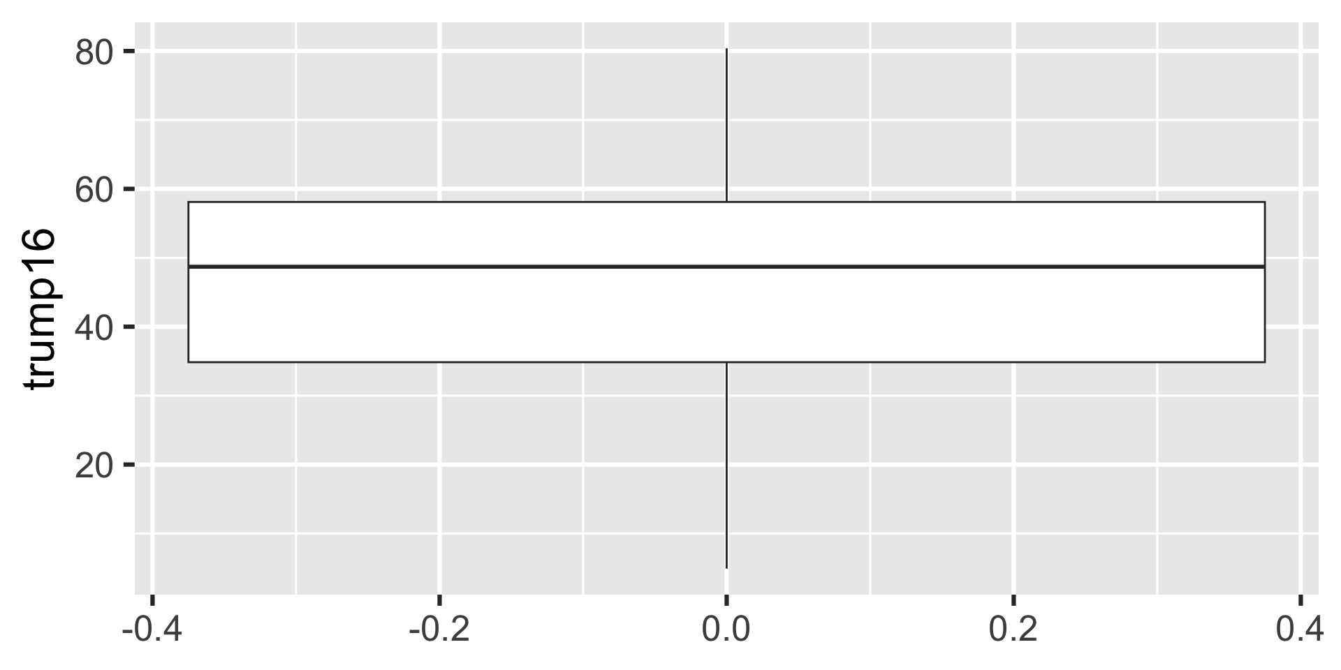
Box plot - Step 1

Box plot - Step 2

Box plot - Step 3
Box plot - Alternative Step 2 + 3
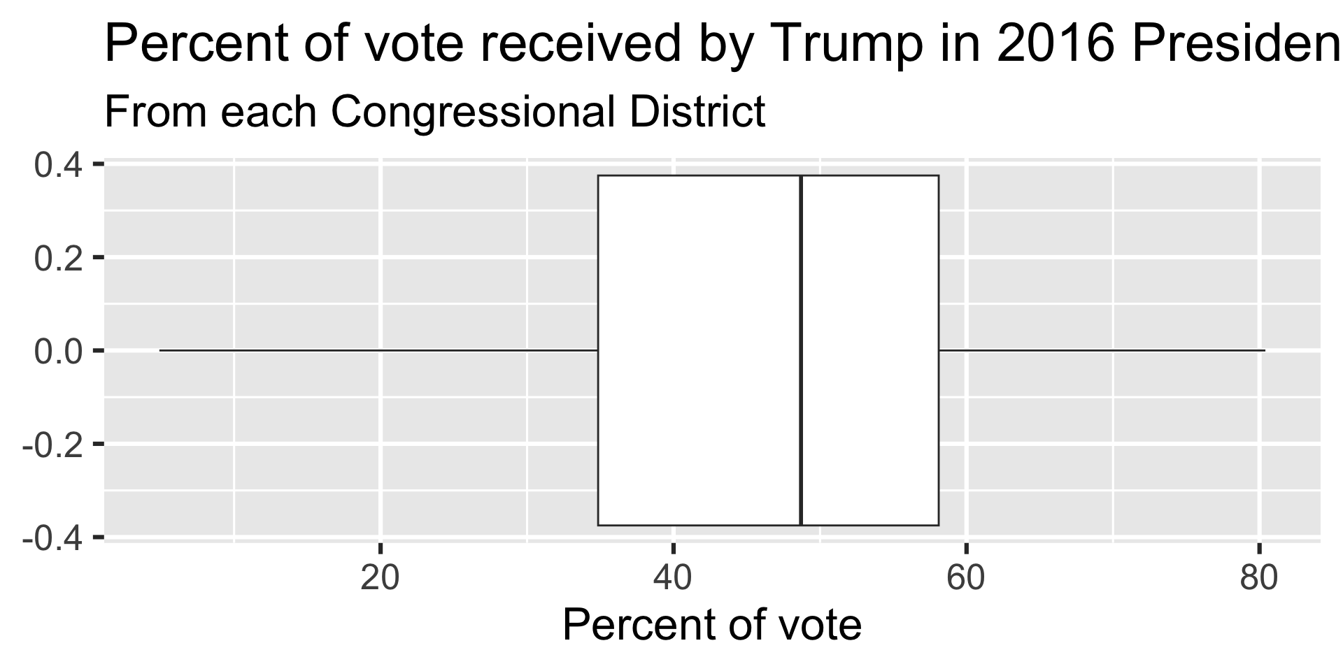
Box plot - Step 4
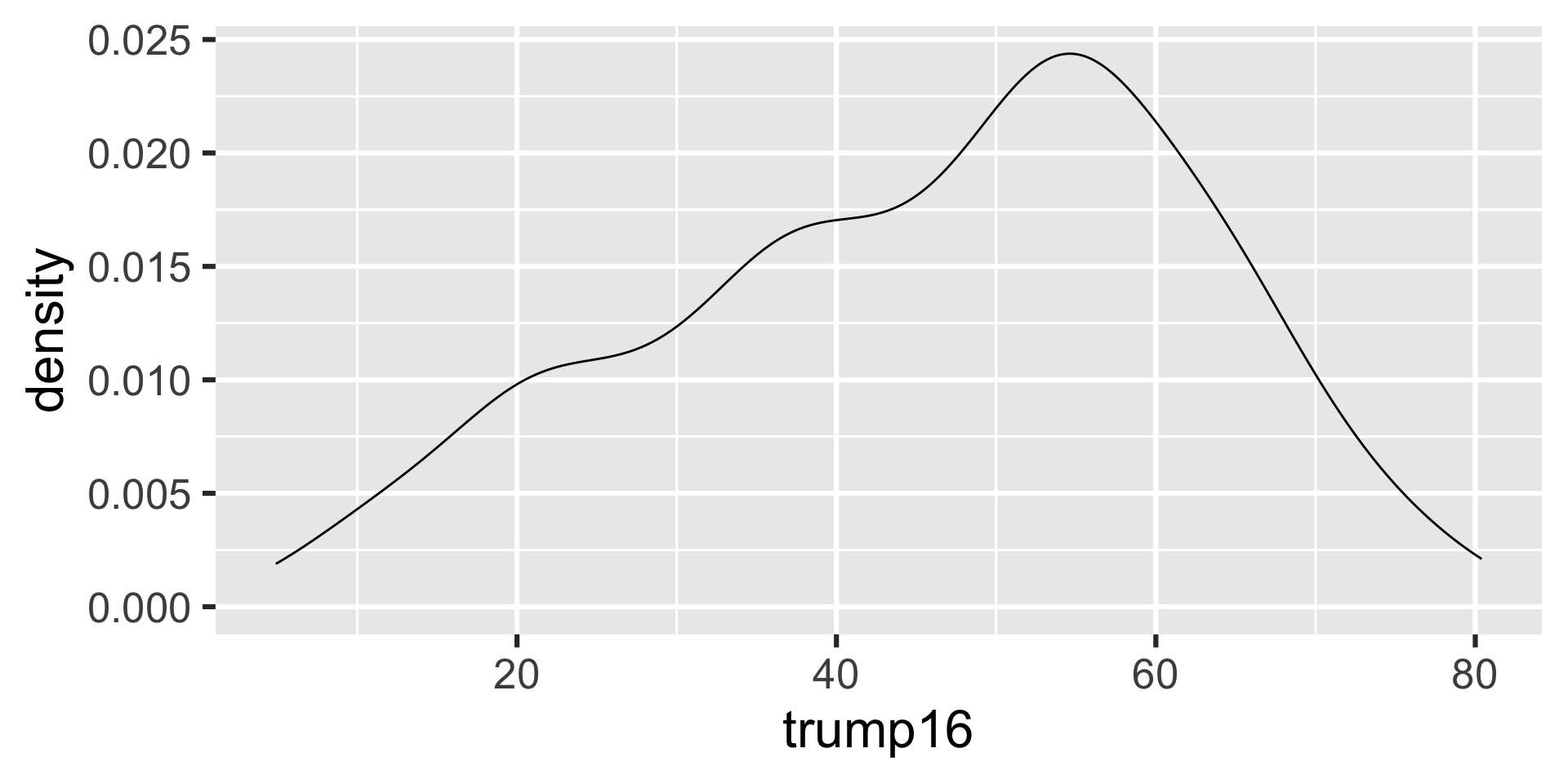
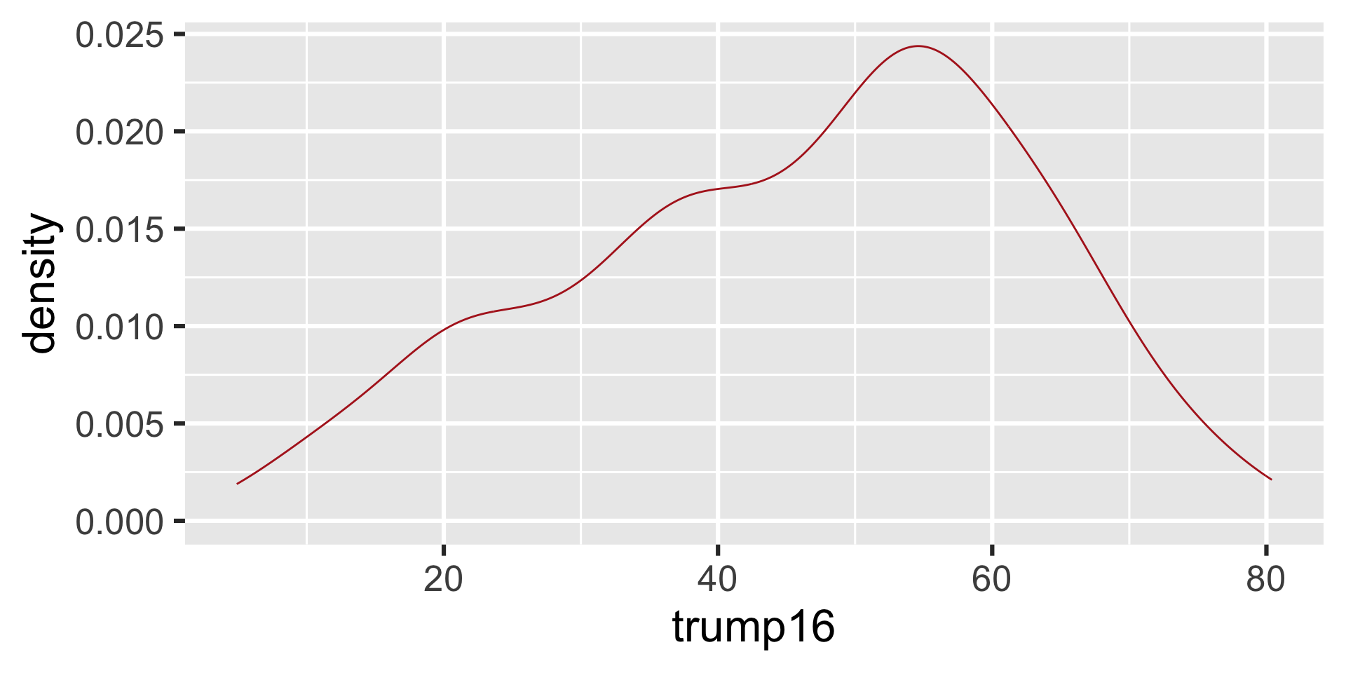
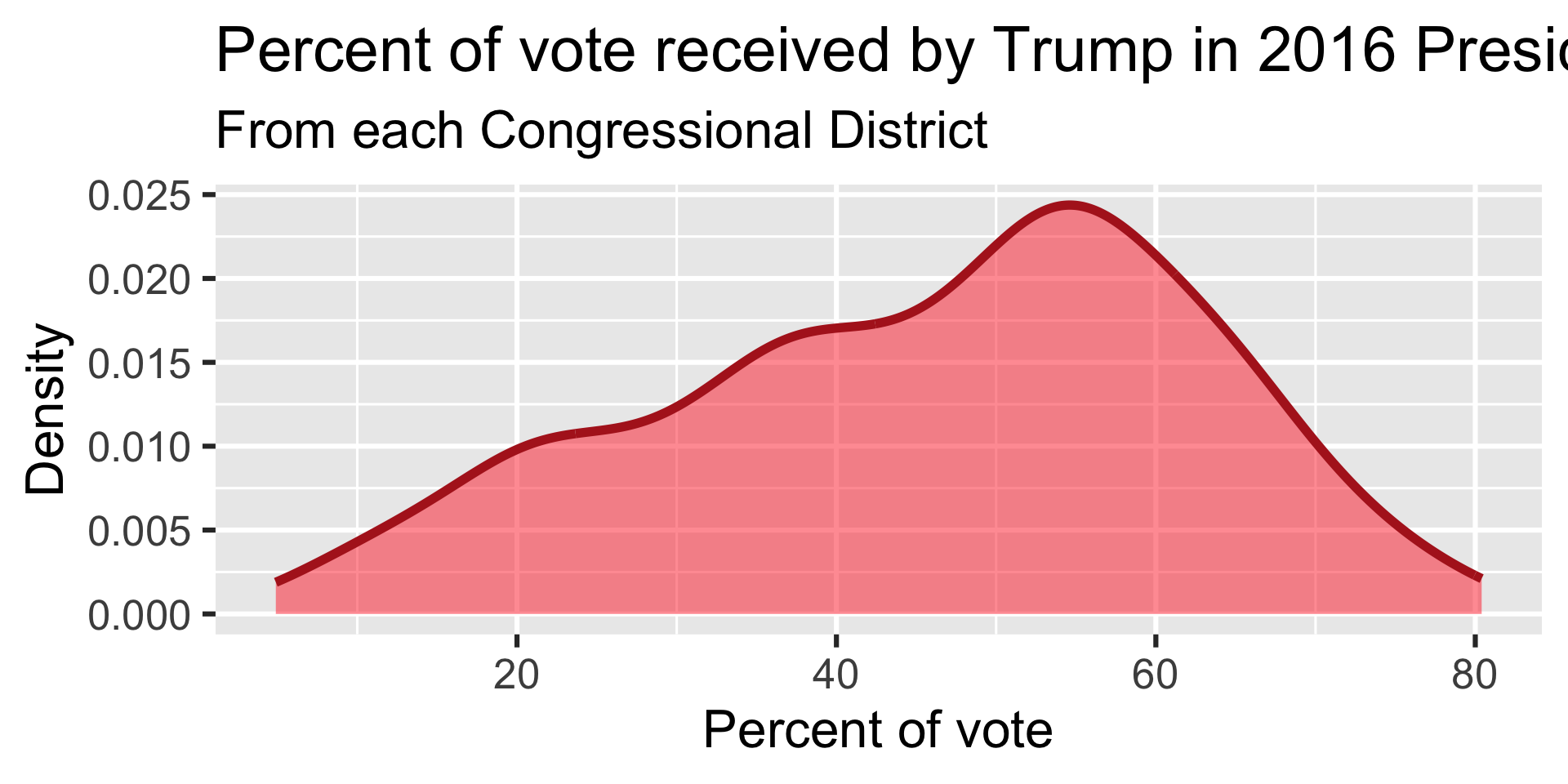
Density plot - Step 1

Density plot - Step 2
Density plot - Step 3
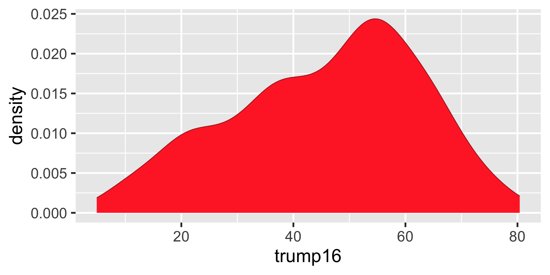
Density plot - Step 4
Density plot - Step 5
Density plot - Step 6
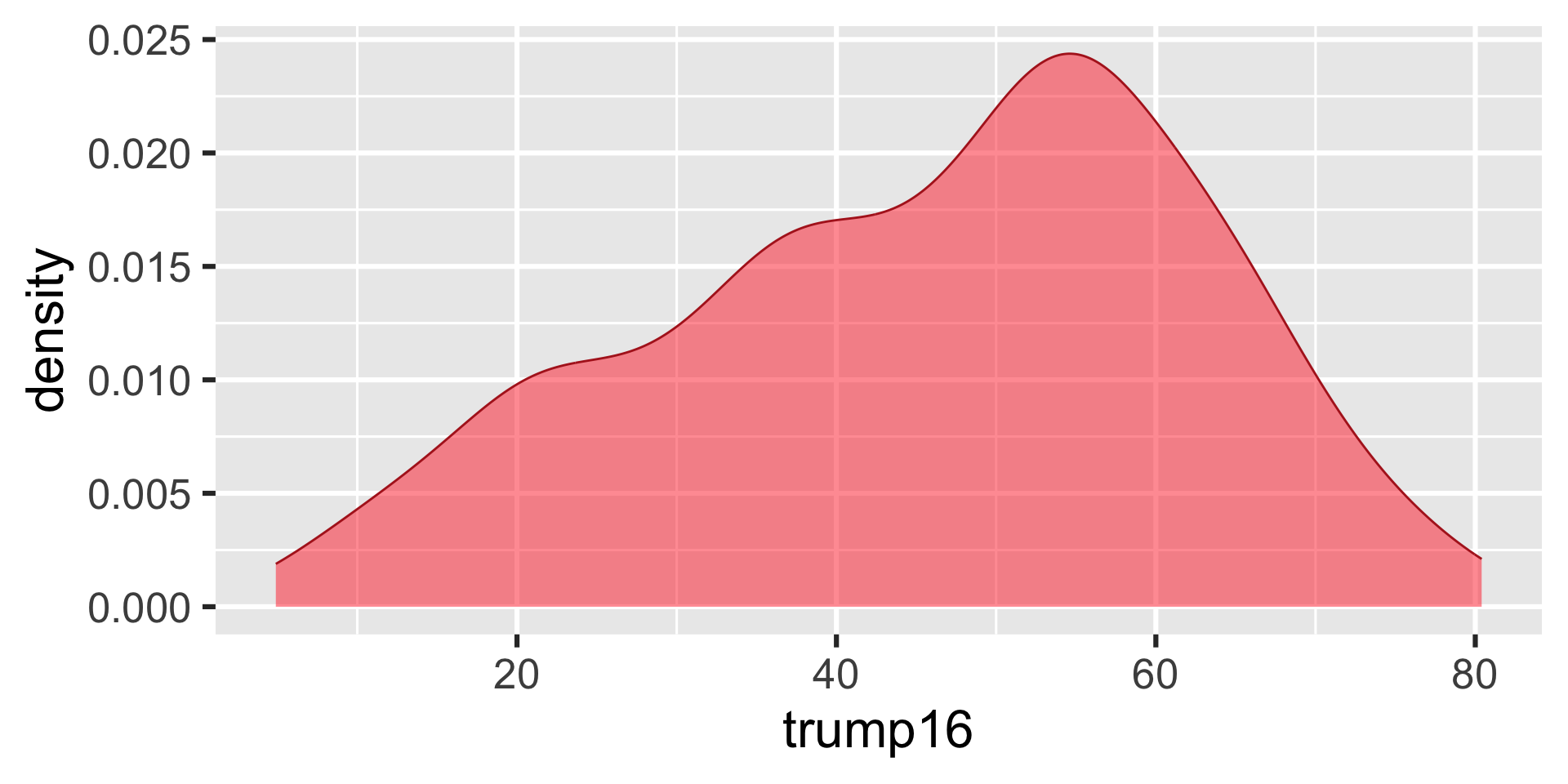
Density plot - Step 7
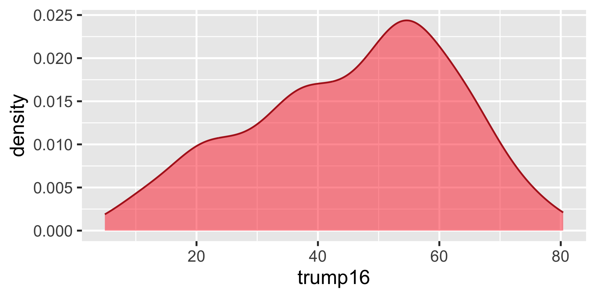
Density plot - Step 8
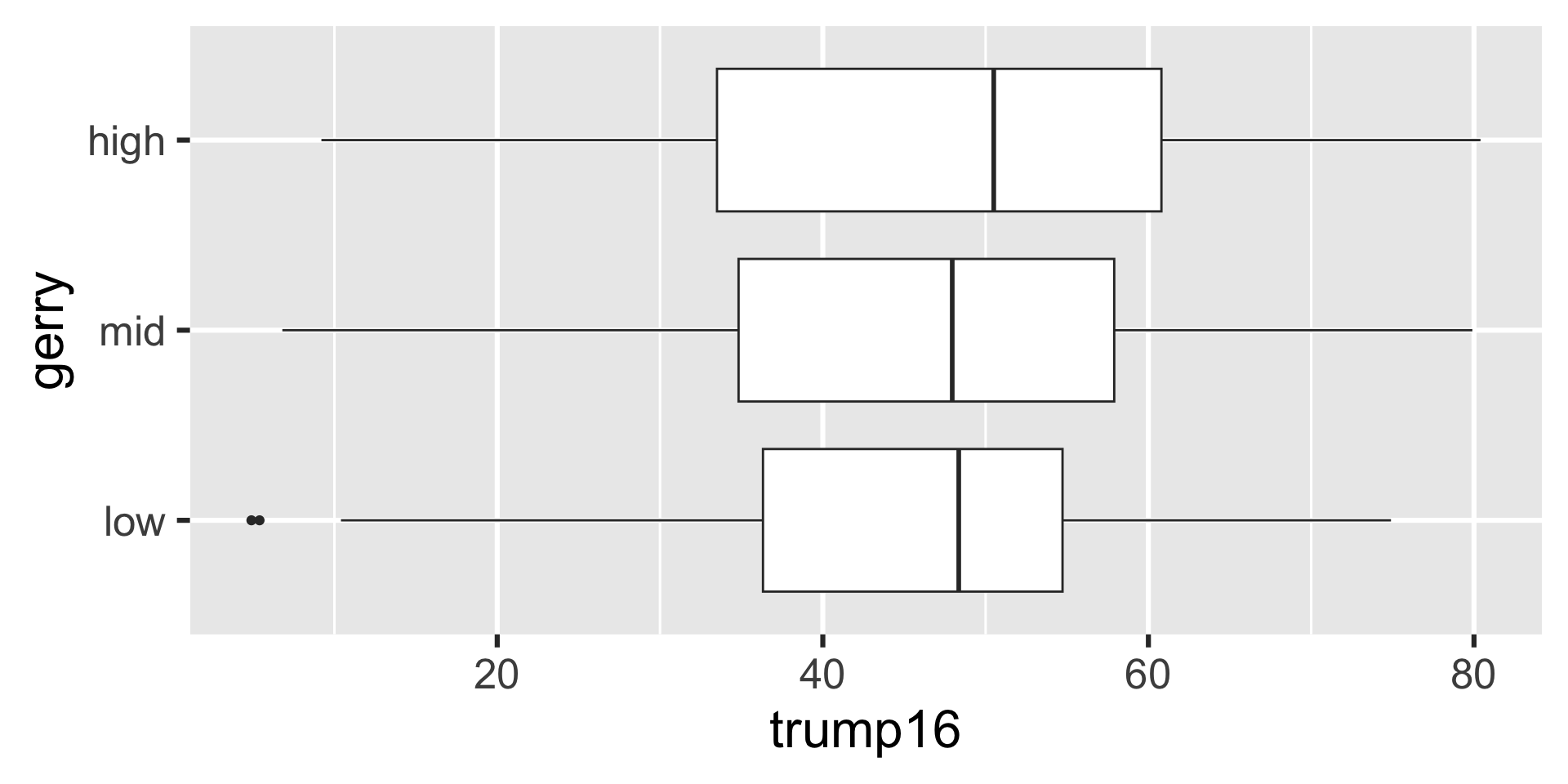
Side-by-side box plots
Participate 📱💻
What goes in the [blank] in the code below to do the following step for each level of gerry?
Scan the QR code or go to app.wooclap.com/sta199. Log in with your Duke NetID.
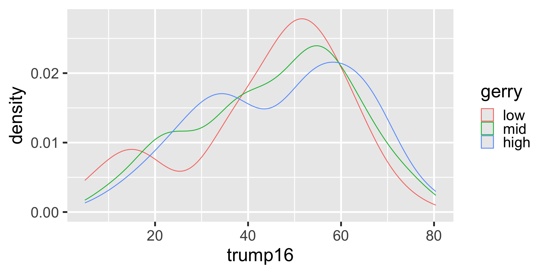
Density plots
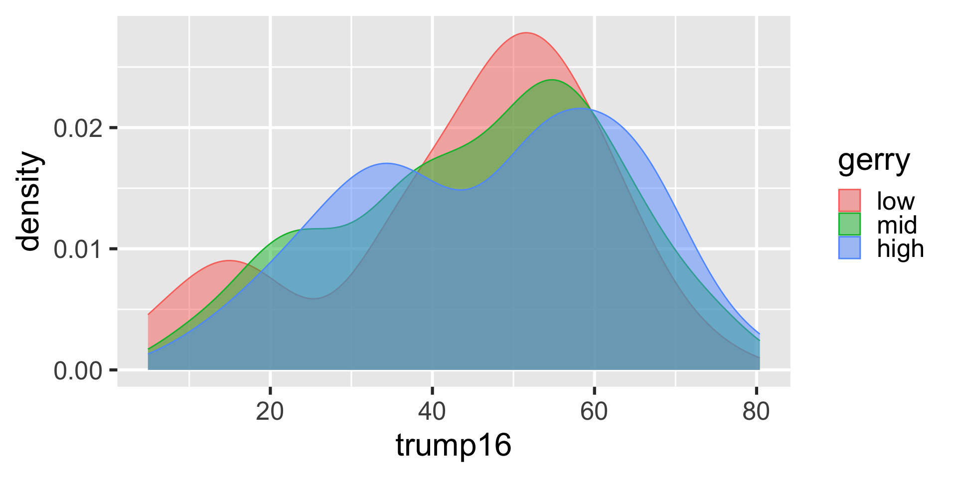
Filled density plots
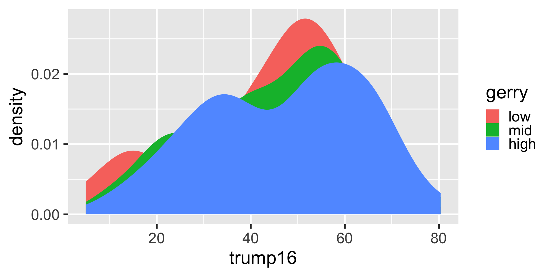
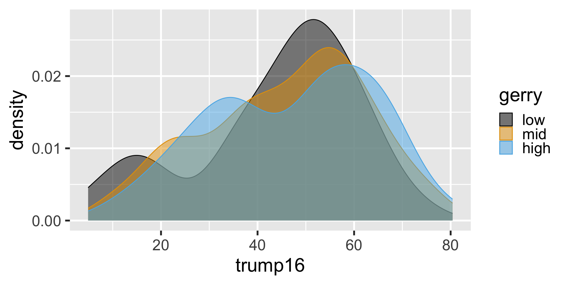
Better filled density plots
Better colors
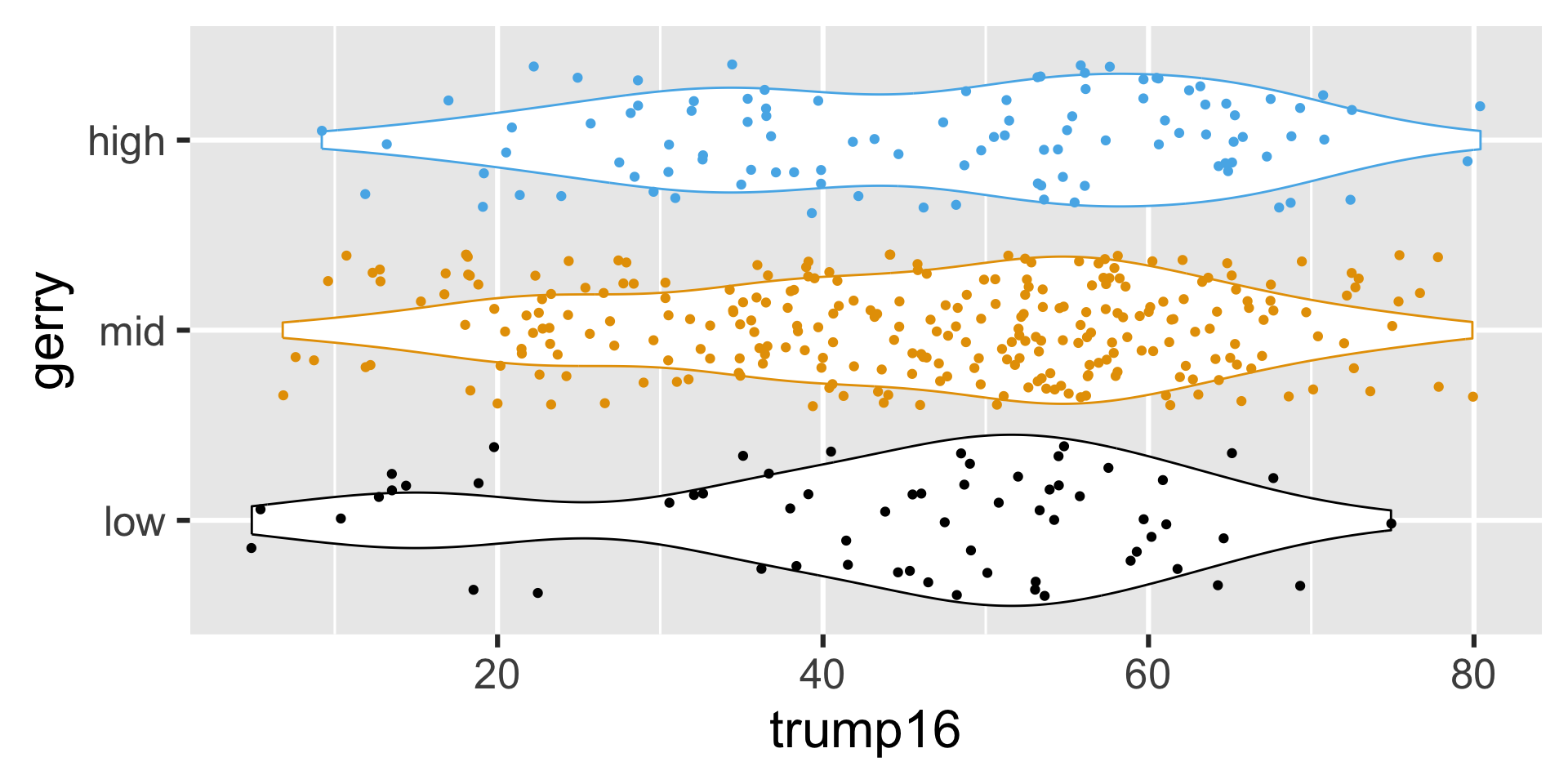
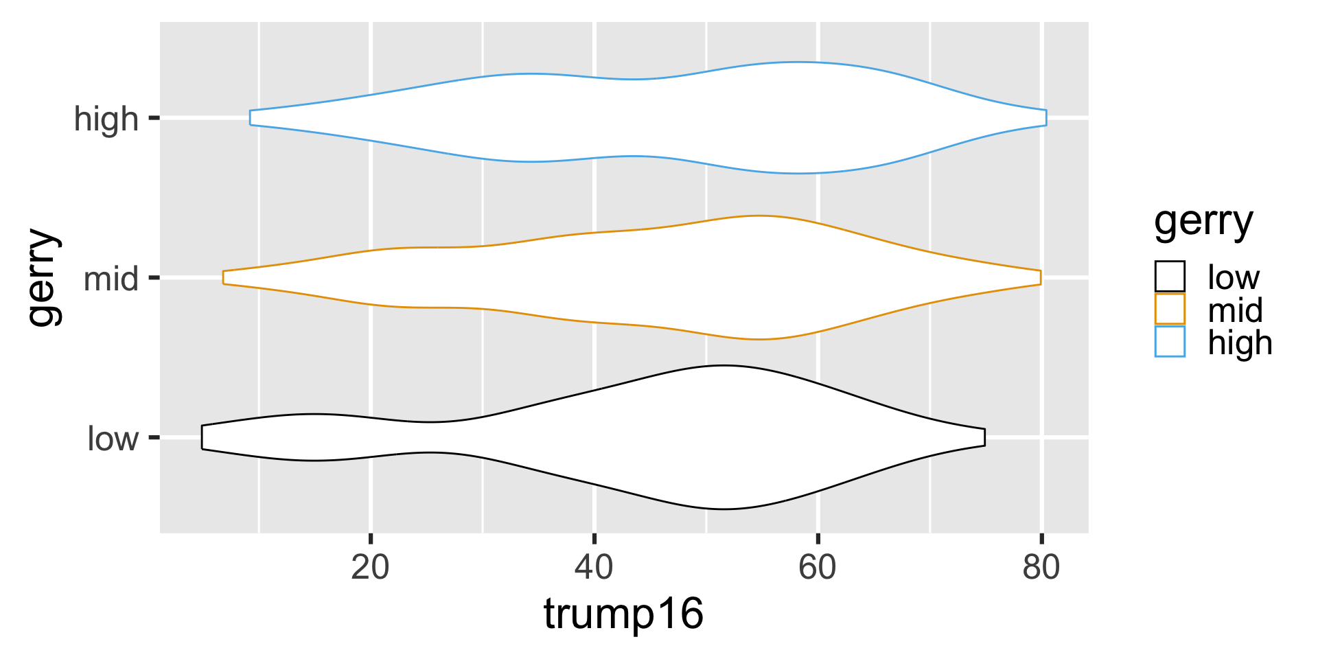
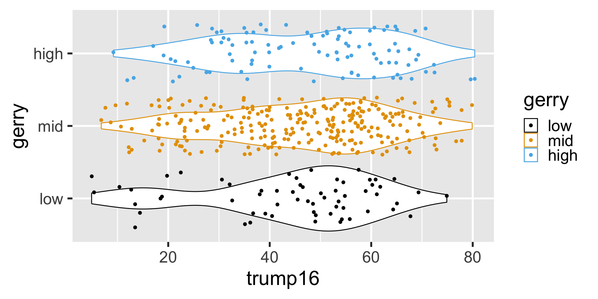
Violin plots
Multiple geoms
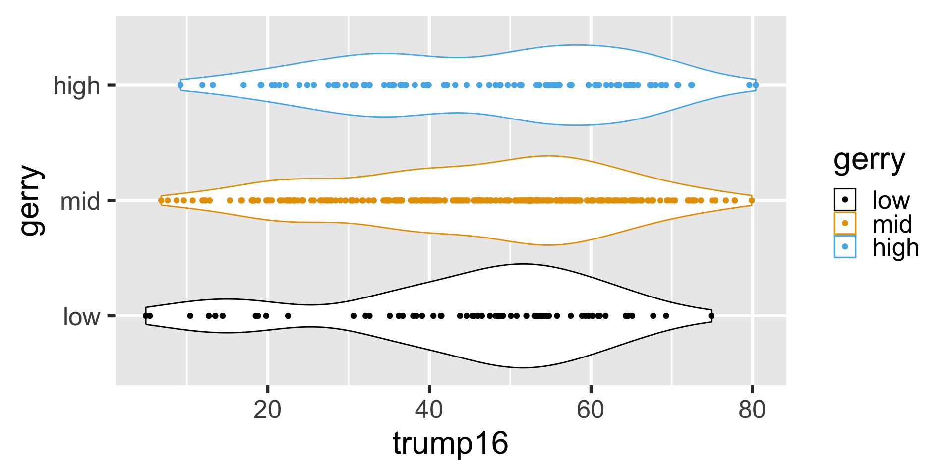
Multiple geoms
Remove legend