Looking further
Lecture 26
Warm-up
Give feedback!
Take 2 minutes to fill out the TA evaluation form – link in your email! Due Monday, December 8th.
Nominate a TA for the StatSci TA of the Year award by sending an email to dus@stat.duke.edu with a brief narrative for your nomination.


- Please also fill out the course evaluation (on DukeHub) as well, I’d love to your feedback!
Announcements
-
HW 6:
- Q4: Instructions clarified – save result as
births14 - Q8: Table to recreate updated
- Q4: Instructions clarified – save result as
Final exam review: Tuesday, Dec 9, 3-4 pm at Soc Sci 136
Final exam office hourse posted
Extra credit
Due: On paper (hand written or typed) at the final exam review
Task:
Write one question for the final exam.
Must be related to course content, which specific references from course content (lecture slide deck, book chapter, video, etc.)
Can be a 3-point (one correct answer) or 5-point (select-all-that-apply) question
Grading:
If you turn in a “good” (or good enough) question, you get +1 or +2 points on your Exam 2, depending on the quality of the question.
I will use one of these questions on the exam, so that’s even more incentive to write a really good one!
If you turn in a “not good enough” question, you don’t get any extra credit.
Awards
Best ugly plot
Best team name
Most messed up repo
From last time
Participate 📱💻
p-value is the probability of ___
- accepting the null hypothsesis
- null hypothesis being true
- observed or more extreme outcome given that the null hypothesis is true
- null hypothesis being true given the outcome
- a false positive

Scan the QR code or go to app.wooclap.com/sta199. Log in with your Duke NetID.
Decision making with hypothesis tests
Setup
Sex discrimination in hiring
A study investigating sex discrimination in the 1970s was set in the context of personnel decisions within a bank. The research question we hope to answer is, “Are individuals who identify as female discriminated against in promotion decisions made by their managers who identify as male?”
This study considered sex roles, and only allowed for options of “male” and “female”. The identities being considered are not gender identities and the study allowed only for a binary classification of sex.
Rosen, B., and T. H. Jerdee. 1974. “Influence of Sex Role Stereotypes on Personnel Decisions.” Journal of Applied Psychology 59 (1): 9. https://doi.org/doi.org/10.1037/h0035834.
Study design
Participants: 48 bank supervisors who identified as male, attending a management institute at the University of North Carolina in 1972
Task: Assume the role of the personnel director of a bank and judge whether a candidate should be promoted to a branch manager position based on personnel files they were randomly assigned
Personnel files: Identical except that half of them indicated the candidate identified as male and the other half indicated the candidate identified as female
Variables:
sex(male or female),decision(promoted or not promoted)
Participate 📱💻
Which of the following is the correct null hypothesis for this study?
- Sex and promotion decision are independent
- Sex and promotion decision are dependent
- Males are more likely to be promoted
- Females are more likely to be promoted
- Males and females are equally likely to be promoted
Scan the QR code or go to app.wooclap.com/sta199. Log in with your Duke NetID.
Participate 📱💻
Which of the following is the correct alternative hypothesis for this study?
- Males are more likely to be promoted
- Females are more likely to be promoted
- Males and females are equally likely to be promoted
- Males and females are not equally likely to be promoted
Scan the QR code or go to app.wooclap.com/sta199. Log in with your Duke NetID.
Hypotheses
p = Proportion of candidates promoted
. . .
Null hypothesis: Sex and promotion decision are independent, i.e., males and females are equally likely to be promoted.
\[ p_{Male} = p_{Female} \]
Alternative hypothesis: Sex and promotion decision are dependent, i.e., males and females are not equally likely to be promoted.
\[ p_{Male} \ne p_{Female} \]
Data
sex_discrimination |>
  count(decision, sex) |>
  pivot_wider(
    names_from = decision,
    values_from = n
  ) |>
  mutate(
    total = promoted + `not promoted`,
    p_prmtd = promoted / total
  )
# A tibble: 2 × 5
sex promoted `not promoted` total p_prmtd
<fct> <int> <int> <int> <dbl>
1 male 21 3 24 0.875
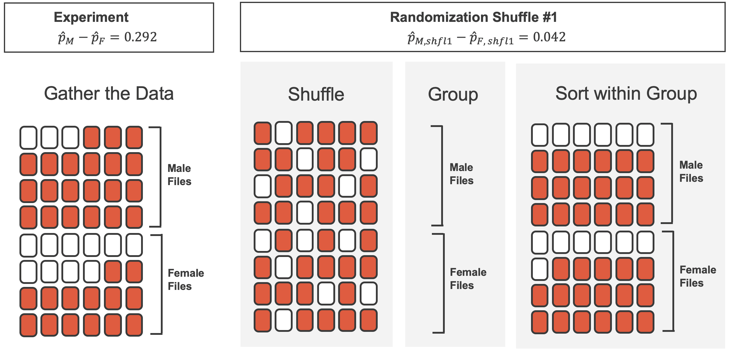
2 female 14 10 24 0.583Observed difference in promotion rates
(male - female)
= 0.875 - 0.583
= 0.292
Simulating under the null
Observed
obs_diff <- sex_discrimination |>
  specify(decision ~ sex, success = "promoted") |>
  calculate(
    stat = "diff in props",
    success = "promoted",
    order = c("male", "female")
  )

obs_diff
Response: decision (factor)
Explanatory: sex (factor)
# A tibble: 1 × 1
stat
<dbl>
1 0.292Null distribution
set.seed(199)
null_dist <- sex_discrimination |>
  specify(decision ~ sex, success = "promoted") |>
  hypothesize(null = "independence") |>
  generate(reps = 10000, type = "permute") |>
  calculate(
    stat = "diff in props",
    success = "promoted",
    order = c("male", "female")
  )

null_dist
Response: decision (factor)
Explanatory: sex (factor)
Null Hypothes...
# A tibble: 10,000 × 2
replicate stat
<int> <dbl>
1 1 -0.208
2 2 0.125
3 3 -0.0417
4 4 -0.0417
5 5 0.125
6 6 -0.125
7 7 -0.0417
8 8 -0.0417
9 9 -0.0417
10 10 -0.0417
# ℹ 9,990 more rowsVisualizing the null distribution
visualize(null_dist)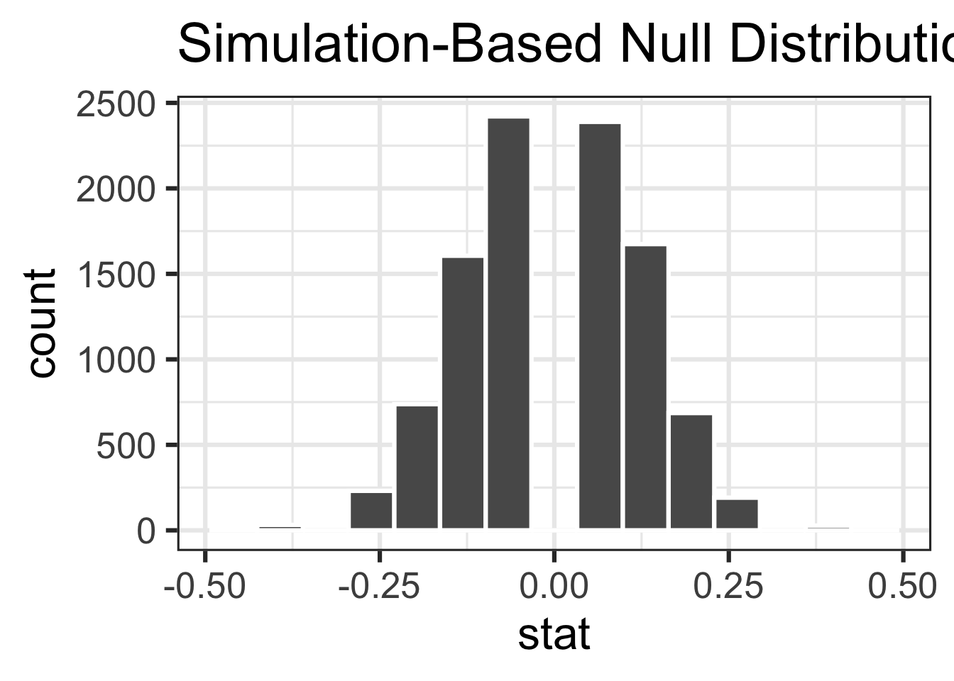
Visualizing the p-value
visualize(null_dist) +
  shade_p_value(obs_stat = obs_diff, direction = "two-sided")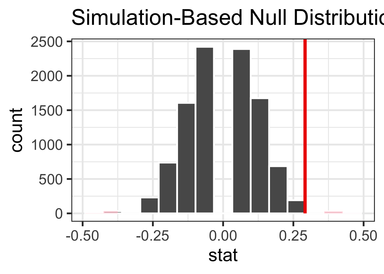
Calculating the p-value
get_p_value(
  null_dist,
  obs_stat = obs_diff,
  direction = "two-sided"
)
# A tibble: 1 × 1
p_value
<dbl>
1 0.044Conclusion
With a p-value smaller than 0.05, we reject the null hypothesis and conclude that the data provide convincing evidence of a discernible difference between the male and female promotion rate, i.e., sex discrimination in promotion decisions.
Decision making, the Bayesian way
What’s the chance of winning?
What is the probability of getting an outcome \(\ge\) 4 when rolling a 6-sided die? What is the probability when rolling a 12-sided die?
- 6-sided: \(\frac{3}{4}\), 12-sided: \(\frac{1}{2}\)
- 6-sided: \(\frac{1}{3}\), 12-sided: \(\frac{2}{3}\)
- 6-sided: \(\frac{1}{2}\), 12-sided: \(\frac{3}{4}\)
- 6-sided: \(\frac{2}{3}\), 12-sided: \(\frac{1}{3}\)
Which die is the good die?
You’re playing a game where you win if the die roll is \(\ge\) 4. If you could get your pick, which die would you prefer to play this game with?
- 6-sided
- 12-sided
Interpretation of probability
- Frequentist interpretation:
- The probability of an outcome is the proportion of times the outcome would occur if we observed the random process an infinite number of times.
- Single main stream school until recently.
- What we’ve been using so far in this course.
- Bayesian interpretation:
- A Bayesian interprets probability as a subjective degree of belief: For the same event, two separate people could have differing probabilities.
- Largely popularized by revolutionary advance in computational technology and methods during the last twenty years.
Set up
I have two dice: one 6-sided, the other 12-sided.
We’re going to play a game where I’m going to call them die A and die B, and you won’t know which one is which.
You pick die A or B, I roll it, and I tell you if you win or not, where winning is getting a number \(\ge\) 4. If you win, you get a piece of candy. If you lose, I get to keep the candy.
We’ll play this multiple times with different contestants.
I will not swap die A and B at any point.
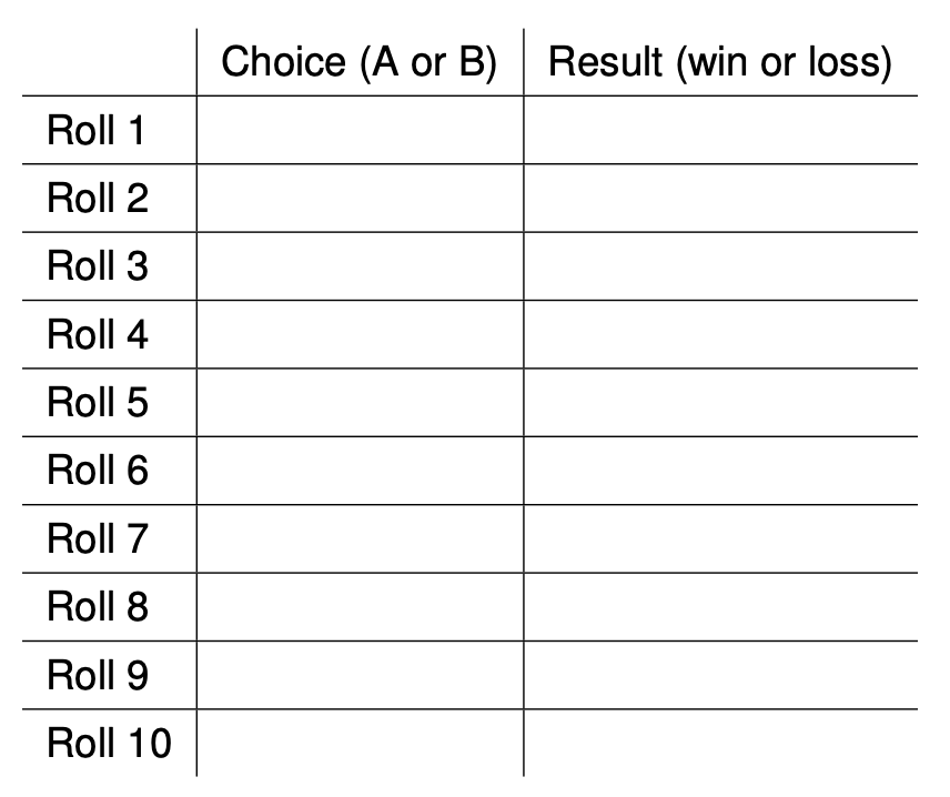
We’ll record which die each contestant picks and whether they won or lost.
The ultimate goal is to come to a class consensus about whether A or B is the good die.
You get to pick how long you want to keep playing, but remember, each time you guess wrong, you lose a piece of candy (so there is a cost associated with too many tries). If you make the wrong decision, you lose all the candy.
Hypotheses and decisions
Sampling isn’t free!
At each trial you risk losing pieces of candy if you lose (the die comes up \(<\) 4). Too many trials means you won’t have much candy left. And if we spend too much class time and we may not get through all the material.
Initial guess
You have no idea if I have chosen A to be the good die (12-sided) or bad die (6-sided). Then, before we collect any data, what is your best guess for A is the good die and B is the bad die?
- P(A good, B bad) = 0.33; P(A bad, B good) = 0.67
- P(A good, B bad) = 0.50; P(A bad, B good) = 0.50
- P(A good, B bad) = 0; P(A bad, B good) = 1
- P(A good, B bad) = 0.25; P(A bad, B good) = 0.75
Prior probabilities
-
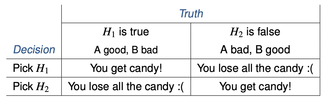
These are your prior probabilities for the two competing claims (hypotheses):
- \(H_1\): A good, B bad
- \(H_2\): A bad, B good
That is, these probabilities represent what you believe before seeing any data.
You could have conceivably made up these probabilities, but instead you have chosen to make an educated guess.
Results
Decision making
What is your decision?
How did you make this decision?
Probability tree - roll 1
What is the probability, based on the outcome of the {first} roll, that A is the good die (and B is the bad die)?
Posterior probability
- The probability
\[ {P(A~is~good~|~outcome~of~1^{st}~roll)} \]
is also called the posterior probability.
Posterior probability is generally defined as P(hypothesis \(|\) data). It tells us the probability of a hypothesis we set forth, given the data we just observed. It depends on both the prior probability we set and the observed data.
This is different than a p-value (a Frequentist concept) which is roughly P(data \(|\) hypothesis).
In the next iteration (roll) we get to take advantage of what we learned from the data.
In other words, we update our prior with our posterior.
Recap: Bayesian inference
Take advantage of prior information, like a previously published study or a physical model.
Naturally integrate data as you collect it, and update your priors.
Avoid the counter-intuitive Frequentist definition of a p-value as the P(observed or more extreme outcome \(|\) \(H_0\) is true). Instead base decisions on the posterior probability, P(hypothesis is true \(|\) observed data).
Watch out! A good prior helps, a bad prior hurts, but the prior matters less the more data you have.
More advanced Bayesian techniques offer flexibility not present in Frequentist models.
And finally…
Thank you!