Cheat sheet: 8.5x11, both sides, hand written or typed, any content you want, must be prepared by you
Bring a pencil and eraser (you’re allowed to use a pen, but you might not want to)
Exam - Take home:
Open book, notes, internet
No office hours
Questions on Ed (private by default)
Due Saturday, November 22 at noon
Reminder: Academic dishonesty / Duke Community Standard
Next Tuesday: Can watch class live on Panopto link
From last class: ae-14-chicago-taxi-classification
Finish up the application exercise by finding the area under the ROC curve.
Recap
Split data into training and testing sets (generally 75/25)
Fit models on training data and reduce to a few candidate models
Make predictions on testing data
Evaluate predictions on testing data using appropriate predictive performance metrics
Linear models: Adjusted R-squared, AIC, etc.
Logistic models: False negative and positive rates, AUC (area under the curve), etc.
Don’t forget to also consider explainability and domain knowledge when selecting a final model
In a future machine learning course: Cross-validation (partitioning training data into training and validation sets and repeating this many times to evaluate model predictive performance before using the testing data), feature engineering, hyperparameter tuning, more complex models (random forests, gradient boosting machines, neural networks, etc.)
Modeling review
Hotel cancellations
library(tidyverse)library(tidymodels)
hotels <-read_csv("data/hotels.csv")
Data prep
Relevel is_canceled
Remove bookings with average daily rate greater than $1,000
Remove bookings with number of adults greater than or equal to 5
Split the data into a training set (75%) and a testing set (25%)
# A tibble: 2 × 3
  term                      estimate exp_estimate
  <chr>                        <dbl>        <dbl>
1 (Intercept)               -0.510          0.601
2 arrival_date_day_of_month -0.00152        0.998
On the 0th day of the month, the odds of reservations being canceled is predicted to be 0.601, on average. The intercept is not meaningful in this context since there is no 0th day of the month.
Prediction in logistic regression
Predict the probability of cancellation for a booking made on the 18th day of the month.
# A tibble: 1 × 1
  .pred_class
  <fct>
1 not canceled
Cancellation ~ arrival date + hotel type
Fit another model to predict whether a reservation was cancelled from arrival_date_day_of_month and hotel type (Resort or City Hotel), allowing the relationship between arrival_date_day_of_month and is_canceled to not vary based on hotel type.
is_canceled_fit_2 <-logistic_reg() |>fit(is_canceled ~ arrival_date_day_of_month + hotel, data = hotels_train)tidy(is_canceled_fit_2)
# A tibble: 3 × 3
  term                      estimate exp_estimate
  <chr>                        <dbl>        <dbl>
1 (Intercept)               -0.315          0.729
2 arrival_date_day_of_month -0.00155        0.998
3 hotelResort Hotel         -0.614          0.541
Holding hotel type constant, for each day the booking is later in the month, the odds of reservations being canceled is predicted to be lower by a factor of 0.998, on average.
# A tibble: 3 × 3
  term                      estimate exp_estimate
  <chr>                        <dbl>        <dbl>
1 (Intercept)               -0.315          0.729
2 arrival_date_day_of_month -0.00155        0.998
3 hotelResort Hotel         -0.614          0.541
Holding arrival day of month constant, the odds of Resort Hotel reservations being canceled is predicted to be lower by a factor of 0.541 compared to City Hotel reservations, on average.
# A tibble: 3 × 3
  term                      estimate exp_estimate
  <chr>                        <dbl>        <dbl>
1 (Intercept)               -0.315          0.729
2 arrival_date_day_of_month -0.00155        0.998
3 hotelResort Hotel         -0.614          0.541
On the 0th day of the month, the odds of City Hotel reservations being canceled is predicted to be 0.729, on average. The intercept is not meaningful in this context since there is no 0th day of the month.
Cancellation ~ arrival date * hotel type
Fit another model to predict whether a reservation was cancelled from arrival_date_day_of_month and hotel type (Resort or City Hotel), allowing the relationship between arrival_date_day_of_month and is_canceled to vary based on hotel type.
is_canceled_fit_3 <-logistic_reg() |>fit(is_canceled ~ arrival_date_day_of_month * hotel, data = hotels_train)tidy(is_canceled_fit_3)
exp(-0.00117) = 0.999: In City Hotels, for each day the booking is later in the month, the odds of reservations being canceled is predicted to be lower by a factor of 0.999, on average.
exp(−0.321) = 0.725: In City Hotels, on the 0th day of the month, the odds of reservations being canceled is predicted to be 0.725, on average. The intercept is not meaningful in this context since there is no 0th day of the month.
exp(-0.00117) = 0.998: In Resort Hotels, for each day the booking is later in the month, the odds of reservations being canceled is predicted to be lower by a factor of 0.998, on average.
exp(−0.321) = 0.401: In Resort Hotels, on the 0th day of the month, the odds of reservations being canceled is predicted to be 0.401, on average. The intercept is not meaningful in this context since there is no 0th day of the month.
Participate 📱💻
Suppose we want to select a final model to predict whether a reservation was cancelled. Which metric would be most appropriate to evaluate the predictive performance of our logistic regression models?
Which model would you select as your final model based on AUC?
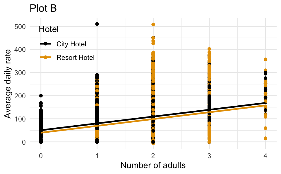
Linear regression
The dataset also contains information about the average daily rate (adr) for each reservation. The following model predicts adr from adults and hotel type.
For each additional Resort Hotel booking, the predicted average daily rate is $10.70 lower, holding number of adults constant.
For each additional adult in the booking, the average daily rate is predicted to be lower by $10.70 for resort hotels compared to City Hotels, on average.
Resort Hotels bookings are predicted to have an average daily rate that is $10.70 lower than City Hotels, on average, holding number of adults constant. ✅
Resort Hotels bookings are predicted to have an average daily rate that is $10.70 higher than City Hotels, on average, holding number of adults constant.