Spending your data

Lecture 21

Dr. Mine Çetinkaya-Rundel

Duke University
STA 199 - Fall 2025

November 11, 2025

Warm-up

While you wait: Participate 📱💻

Which of the following files should you be updating in your project between now and Thursday’s deadline? Check all that apply.

contract.qmd
index.qmd
presentation.qmd or presentation.pdf
proposal.qmd
README.md in your data folder

Scan the QR code or go to app.wooclap.com/sta199. Log in with your Duke NetID.

Announcements

Project write-ups due Thursday at 11:59pm
Peer evaluations due Friday at 11:59pm

From last week

Finish up ae-13-spam-filter.

Setup

Packages

library(tidyverse) # data wrangling and visualization
library(tidymodels) # modeling

Data

Taxi trips in Chicago, IL in 2022
Data from Chicago Data Portal

Data: `chicago_taxi`

chicago_taxi <- read_csv("data/chicago-taxi.csv")

chicago_taxi

# A tibble: 2,000 × 7
   tip   distance company                      local dow   month  hour
   <chr>    <dbl> <chr>                        <chr> <chr> <chr> <dbl>
 1 no        0.4  other                        yes   Fri   Mar      17
 2 no        0.96 Taxicab Insurance Agency Llc no    Mon   Apr       8
 3 no        1.07 Sun Taxi                     no    Fri   Feb      15
 4 no        1.13 other                        no    Sat   Feb      14
 5 no       10.8  Sun Taxi                     no    Sat   Apr      14
 6 no        3.6  Chicago Independents         no    Wed   Mar      12
 7 no        1.08 Flash Cab                    yes   Wed   Mar      13
 8 no        0.85 Taxicab Insurance Agency Llc no    Tue   Mar       8
 9 no       17.9  City Service                 no    Tue   Jan      20
10 no        0    City Service                 yes   Sun   Apr      16
# ℹ 1,990 more rows

Data: `chicago_taxi`

glimpse(chicago_taxi)

Rows: 2,000
Columns: 7
$ tip      <chr> "no", "no", "no", "no", "no", "no", "no", "no", "no…
$ distance <dbl> 0.40, 0.96, 1.07, 1.13, 10.81, 3.60, 1.08, 0.85, 17…
$ company  <chr> "other", "Taxicab Insurance Agency Llc", "Sun Taxi"…
$ local    <chr> "yes", "no", "no", "no", "no", "no", "yes", "no", "…
$ dow      <chr> "Fri", "Mon", "Fri", "Sat", "Sat", "Wed", "Wed", "T…
$ month    <chr> "Mar", "Apr", "Feb", "Feb", "Apr", "Mar", "Mar", "M…
$ hour     <dbl> 17, 8, 15, 14, 14, 12, 13, 8, 20, 16, 20, 8, 15, 15…

Data prep

chicago_taxi <- chicago_taxi |>
  mutate(
    tip = fct_relevel(tip, "no", "yes"),
    local = fct_relevel(local, "no", "yes"),
    dow = fct_relevel(dow, "Mon", "Tue", "Wed", "Thu", "Fri", "Sat", "Sun"),
    month = fct_relevel(month, "Jan", "Feb", "Mar", "Apr")
  )

Outcome and predictors

Outcome - tip: Whether rider left a tip – a factor w/ levels “yes” and “no”
(Potential) predictors:
- Numerical:
  - distance: The trip distance, in odometer miles.
  - hour: The hour of the day in which the trip began.
- Categorical:
  - company: The taxi company – companies that occurred few times were binned as “other”.
  - local: Whether the trip started in the same community area as it began.
  - dow: The day of the week in which the trip began.
  - month: The month in which the trip began.

Should we include a predictor?

To determine whether we should include a predictor in a model, we should start by asking:

Is it ethical to use this variable? (Or even legal?)
Will this variable be available at prediction time?
Does this variable contribute to explainability?

Data splitting and spending

We’ve been cheating!

So far, we’ve been using all the data we have for building models. In predictive contexts, this would be considered cheating.
Evaluating model performance for predicting outcomes that were used when building the models is like evaluating your learning with questions whose answers you’ve already seen.

Spending your data

For predictive models (used primarily in machine learning), we typically split data into training and test sets:

The training set is used to estimate model parameters.
The test set is used to find an independent assessment of model performance.

Warning

Do not use, or even peek at, the test set during training.

How much to spend?

The more data we spend (use in training), the better estimates we’ll get.
Spending too much data in training prevents us from computing a good assessment of predictive performance.
Spending too much data in testing prevents us from computing a good estimate of model parameters.

The initial split

set.seed(20251111)
chicago_taxi_split <- initial_split(chicago_taxi)
chicago_taxi_split

<Training/Testing/Total>
<1500/500/2000>

Setting a seed

What does set.seed() do?

To create that split of the data, R generates “pseudo-random” numbers: while they are made to behave like random numbers, their generation is deterministic given a “seed”.
This allows us to reproduce results by setting that seed.
Which seed you pick doesn’t matter, as long as you don’t try a bunch of seeds and pick the one that gives you the best performance.

Accessing the data

chicago_taxi_train <- training(chicago_taxi_split)
chicago_taxi_test <- testing(chicago_taxi_split)

The training set

chicago_taxi_train

# A tibble: 1,500 × 7
   tip   distance company                      local dow   month  hour
   <fct>    <dbl> <chr>                        <fct> <fct> <fct> <dbl>
 1 no        7.9  Taxi Affiliation Services    no    Sat   Apr      17
 2 no       10.7  Sun Taxi                     no    Fri   Mar       9
 3 yes       3.4  Taxi Affiliation Services    no    Thu   Mar      20
 4 no        4.7  Taxi Affiliation Services    no    Fri   Jan       9
 5 no       18.6  Taxicab Insurance Agency Llc no    Fri   Feb      15
 6 yes       0.89 other                        yes   Fri   Mar      17
 7 no       17.6  City Service                 no    Wed   Feb      19
 8 no        0.97 Taxicab Insurance Agency Llc yes   Thu   Mar      21
 9 no        0.4  other                        yes   Fri   Mar      17
10 yes       2.2  other                        no    Wed   Apr      10
# ℹ 1,490 more rows

The testing data

🙈

Exploratory data analysis

Initial questions

What’s the distribution of the outcome, tip?
What’s the distribution of numeric variables like distance or hour?
How does the distribution of tip differ across the categorical and numerical variables?

While you wait: Participate 📱💻

Which dataset should we use for the exploration?

The entire data chicago_taxi
The training data chicago_taxi_train
The testing data chicago_taxi_test

Scan the QR code or go to app.wooclap.com/sta199. Log in with your Duke NetID.

`tip`

What’s the distribution of the outcome, tip?

chicago_taxi_train |>
  count(tip) |>
  mutate(prop = n / sum(n))

# A tibble: 2 × 3
  tip       n  prop
  <fct> <int> <dbl>
1 no      586 0.391
2 yes     914 0.609

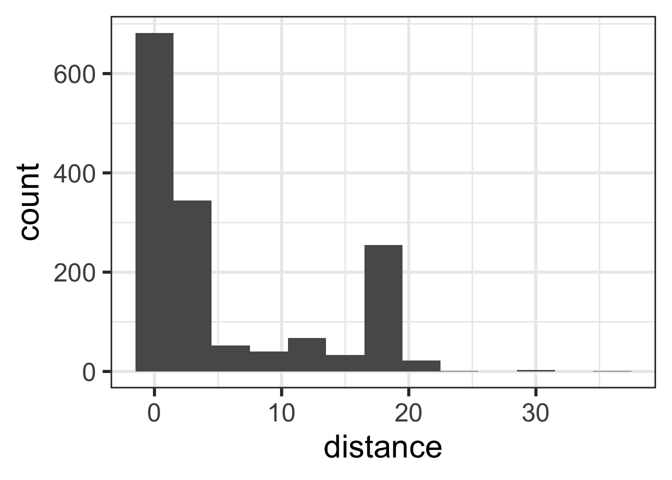
`distance`

What’s the distribution of distance?

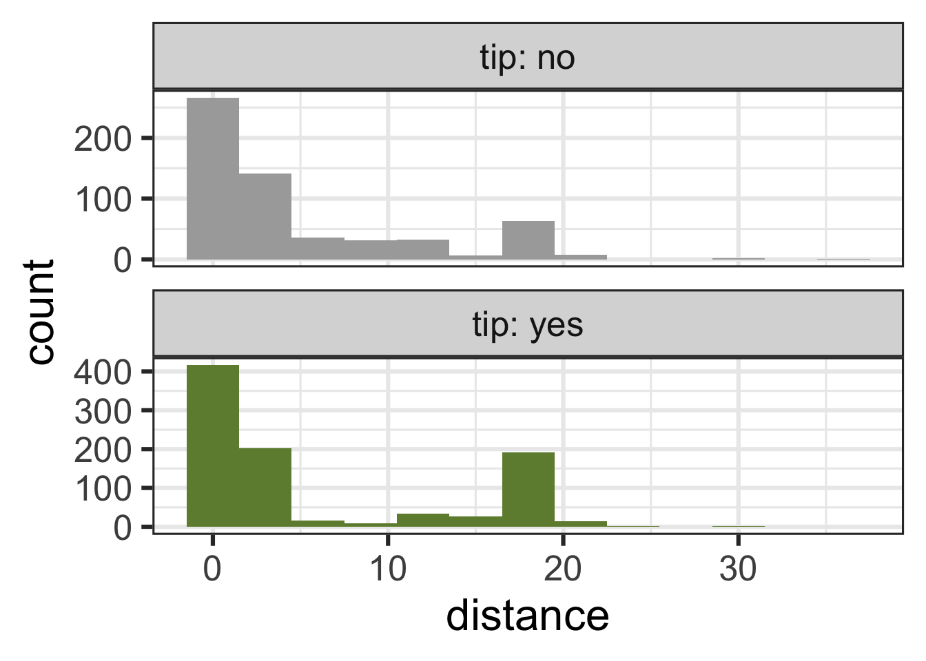
ggplot(chicago_taxi_train, aes(x = distance)) +
  geom_histogram(binwidth = 3)

`tip` and `distance`

ggplot(chicago_taxi_train, aes(x = distance, fill = tip, group = tip)) +
  geom_histogram(binwidth = 3, show.legend = FALSE) +
  scale_fill_manual(values = c("yes" = "darkolivegreen4", "no" = "darkgray")) +
  facet_wrap(~tip, ncol = 1, labeller = label_both, scales = "free_y")

`tip` and `hour`

ggplot(chicago_taxi_train, aes(x = hour, fill = tip, group = tip)) +
  geom_histogram(binwidth = 1, show.legend = FALSE) +
  scale_fill_manual(values = c("yes" = "darkolivegreen4", "no" = "darkgray")) +
  scale_x_continuous(breaks = seq(0, 18, by = 6)) +
  facet_wrap(~tip, ncol = 1, labeller = label_both, scales = "free_y")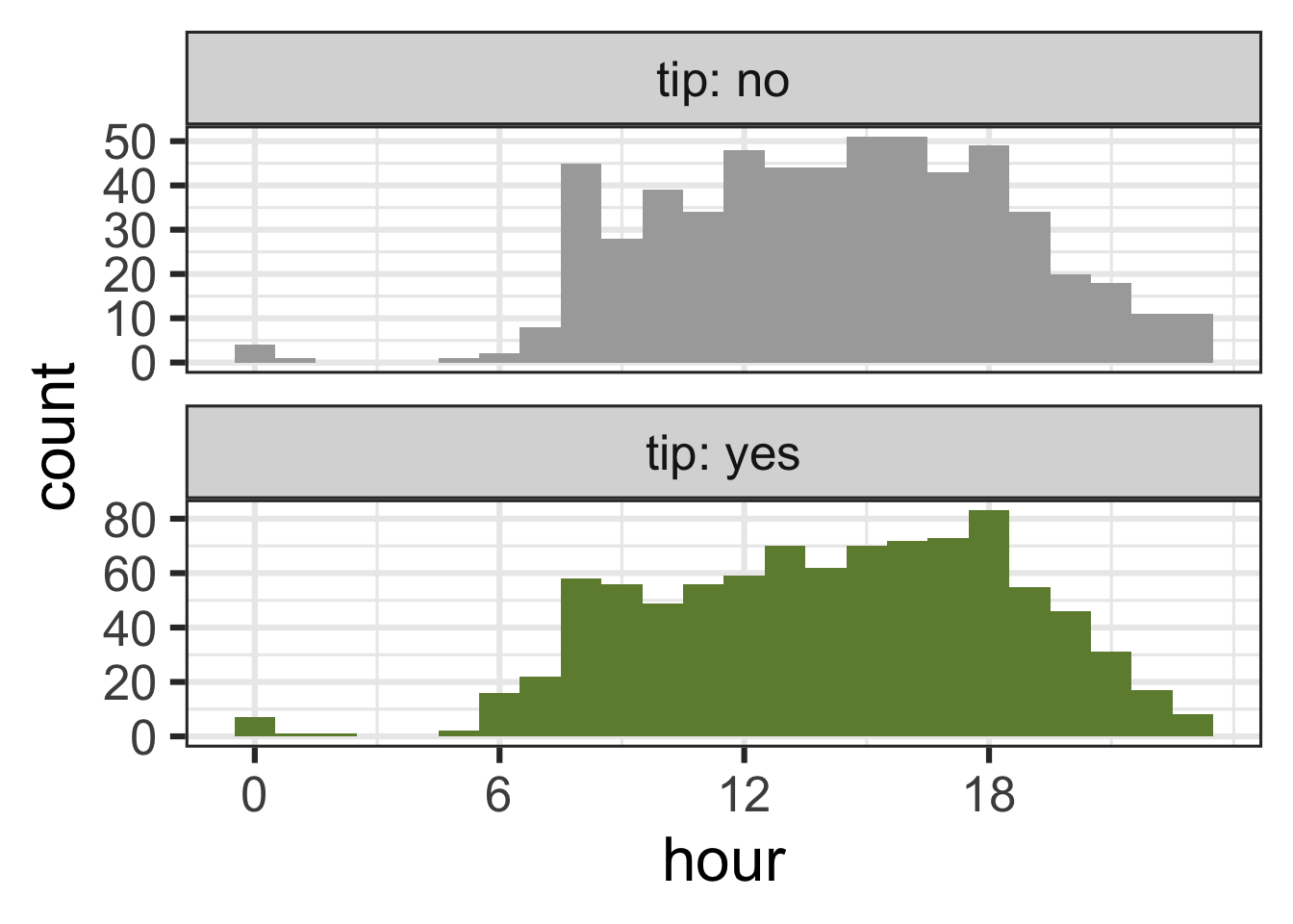

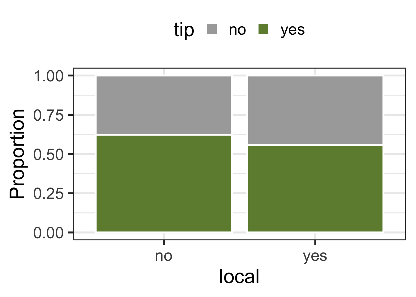
`tip` and `local`

ggplot(chicago_taxi_train, aes(x = local, fill = tip)) +
  geom_bar(position = "fill", color = "white") +
  scale_fill_manual(values = c("yes" = "darkolivegreen4", "no" = "darkgray")) +
  labs(y = "Proportion") +
  theme(legend.position = "top")

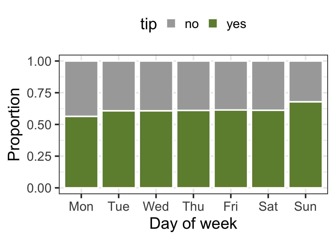
`tip` and `dow`

ggplot(chicago_taxi_train, aes(x = dow, fill = tip)) +
  geom_bar(position = "fill", color = "white") +
  scale_fill_manual(values = c("yes" = "darkolivegreen4", "no" = "darkgray")) +
  labs(y = "Proportion", x = "Day of week") +
  theme(legend.position = "top")

Terminology

False negative and positive

False negative rate is the proportion of actual positives that were classified as negatives.
False positive rate is the proportion of actual negatives that were classified as positives.

Sensitivity

Sensitivity is the proportion of actual positives that were correctly classified as positive.

Also known as true positive rate and recall
Sensitivity = 1 − False negative rate
Useful when false negatives are more “expensive” than false positives

Specificity

Specificity is the proportion of actual negatives that were correctly classified as negative

Also known as true negative rate
Specificity = 1 − False positive rate

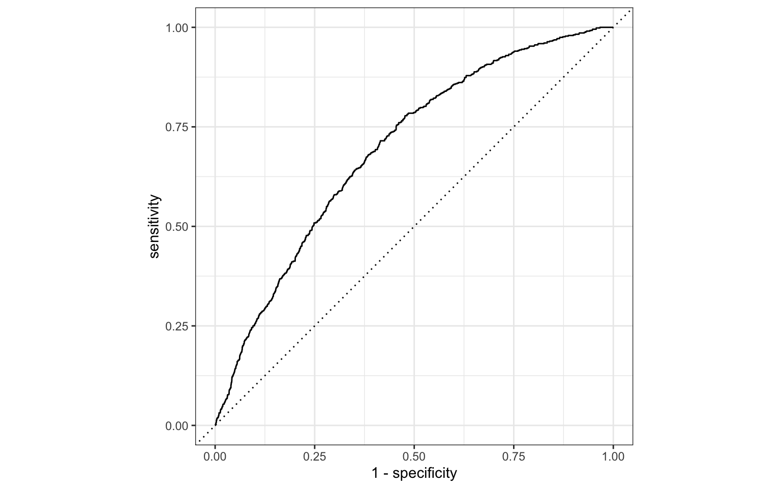
ROC curve

The receiver operating characteristic (ROC) curve allows to assess the model performance across a range of thresholds.

Participate 📱💻

Which of the following best describes the area annotated on the ROC curve?

Where all positives classified as positive, all negatives classified as negative
Where true positive rate = false positive rate
Where all positives classified as negative, all negatives classified as positive

Scan the QR code or go to app.wooclap.com/sta199. Log in with your Duke NetID.

ROC curve

Which corner of the plot indicates the best model performance?

Next steps

Fit models on training data
Make predictions on testing data
Evaluate predictions on testing data:
- Linear models: R-squared, adjusted R-squared, RMSE (root mean squared error), etc.
- Logistic models: False negative and positive rates, AUC (area under the curve), etc.
Make decisions based on model predictive performance, validity across various testing/training splits (aka “cross validation”), explainability

Note

We will only learn about a subset of these in this course, but you can go further into these ideas in STA 210 or STA 221 as well as in various machine learning courses.

ae-14-chicago-taxi-classification

Go to your ae project in RStudio.
If you haven’t yet done so, make sure all of your changes up to this point are committed and pushed, i.e., there’s nothing left in your Git pane.
If you haven’t yet done so, click Pull to get today’s application exercise file: ae-14-chicago-taxi-classification.qmd.
Work through the application exercise in class, and render, commit, and push your edits.

Spending your data

Warm-up

While you wait: Participate 📱💻

Announcements

From last week

Setup

Packages

Data

Data: chicago_taxi

Data: chicago_taxi

Data prep

Outcome and predictors

Should we include a predictor?

Data splitting and spending

We’ve been cheating!

Spending your data

How much to spend?

The initial split

Setting a seed

Accessing the data

The training set

The testing data

Exploratory data analysis

Initial questions

While you wait: Participate 📱💻

tip

distance

tip and distance

tip and hour

tip and local

tip and dow

Terminology

False negative and positive

Sensitivity

Specificity

ROC curve

Participate 📱💻

ROC curve

Next steps

Next steps

ae-14-chicago-taxi-classification

Data: `chicago_taxi`

Data: `chicago_taxi`

`tip`

`distance`

`tip` and `distance`

`tip` and `hour`

`tip` and `local`

`tip` and `dow`