Linear models with a single predictor

Lecture 16

Author

Affiliation

Dr. Mine Çetinkaya-Rundel

Duke University
STA 199 - Fall 2025

Published

October 23, 2025

Warm-up

While you wait: Participate 📱💻

Play the game a few times and report your score: smallest absolute difference between your guess and the actual correlation, e.g., if the actual correlation was 0.8 and you guessed 0.6, your score would be 0.2. If the actual correlation was -0.4 and you guessed 0.1, your score would be 0.5.

Option 1 - Calculates your score for you: https://duke.is/corr-game-1
Option 2 - You need to calculate your own score: https://duke.is/corr-game-2

Scan the QR code or go to app.wooclap.com/sta199. Log in with your Duke NetID.

Announcements

Peer evaluation 2 due on tonight at 11:59 pm – see email from TEAMMATES.
Make progress on projects – any questions?

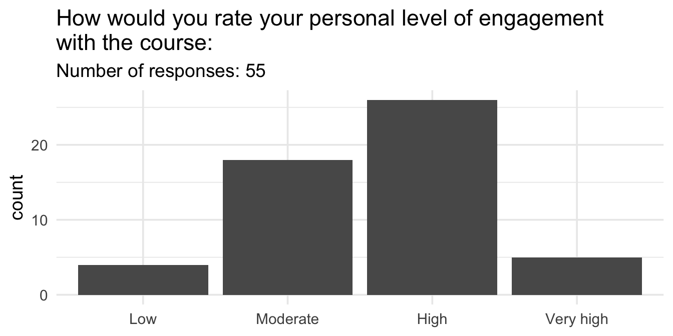
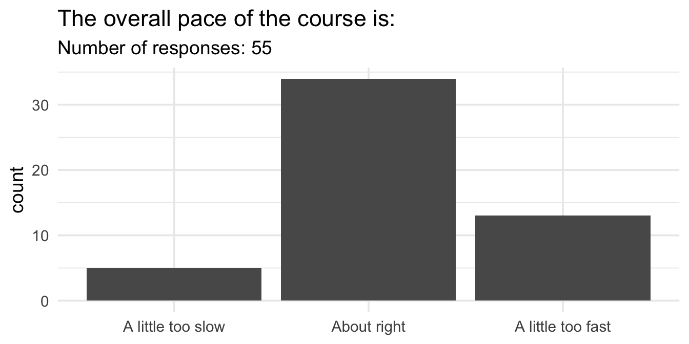
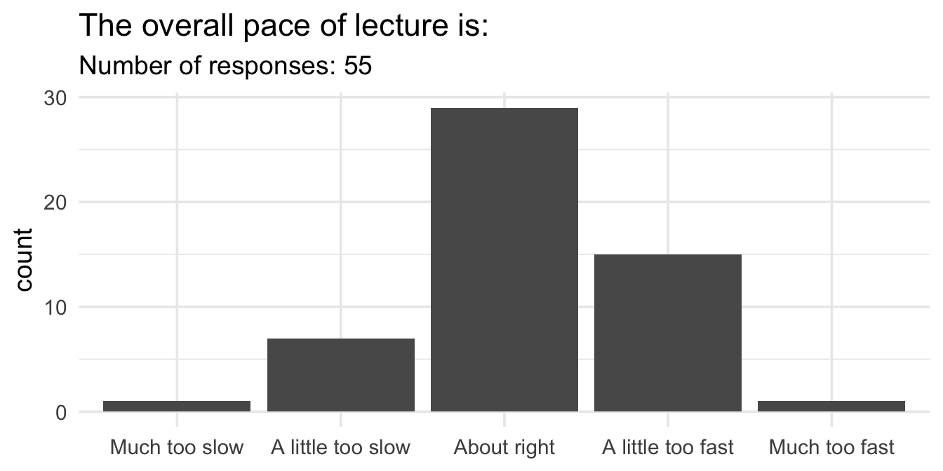
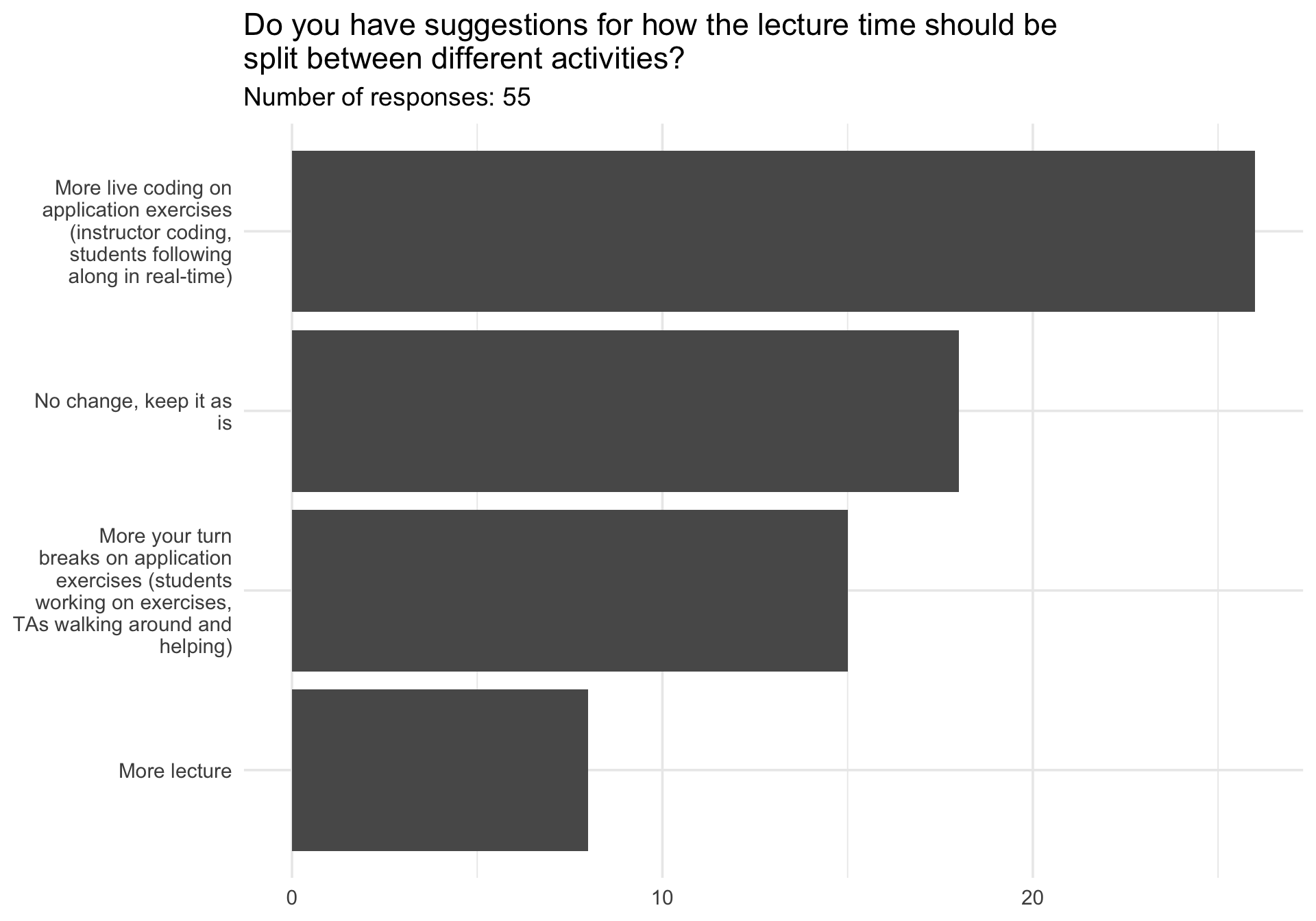
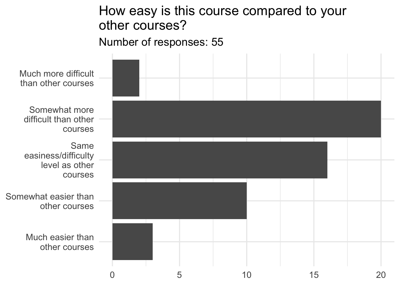
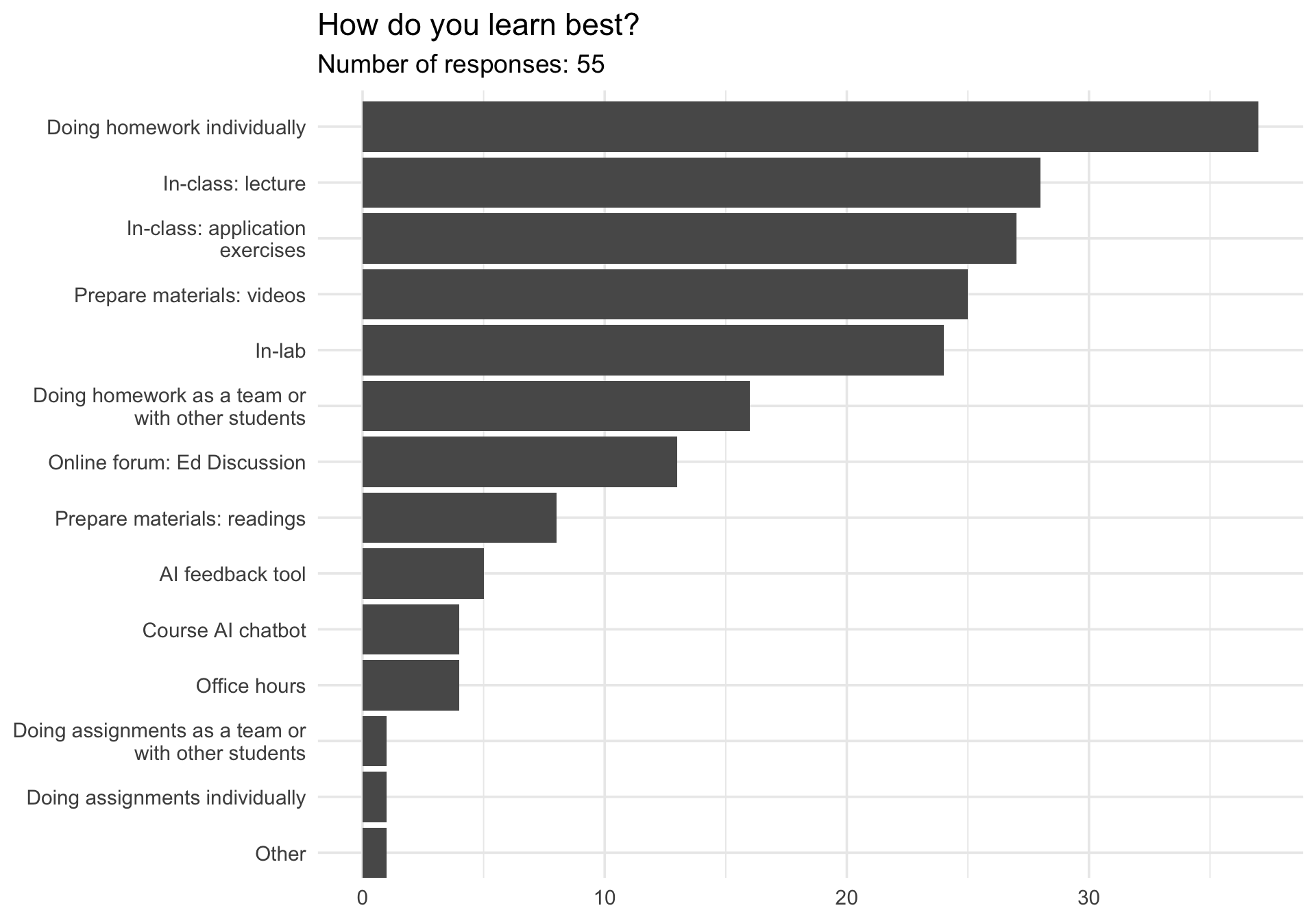
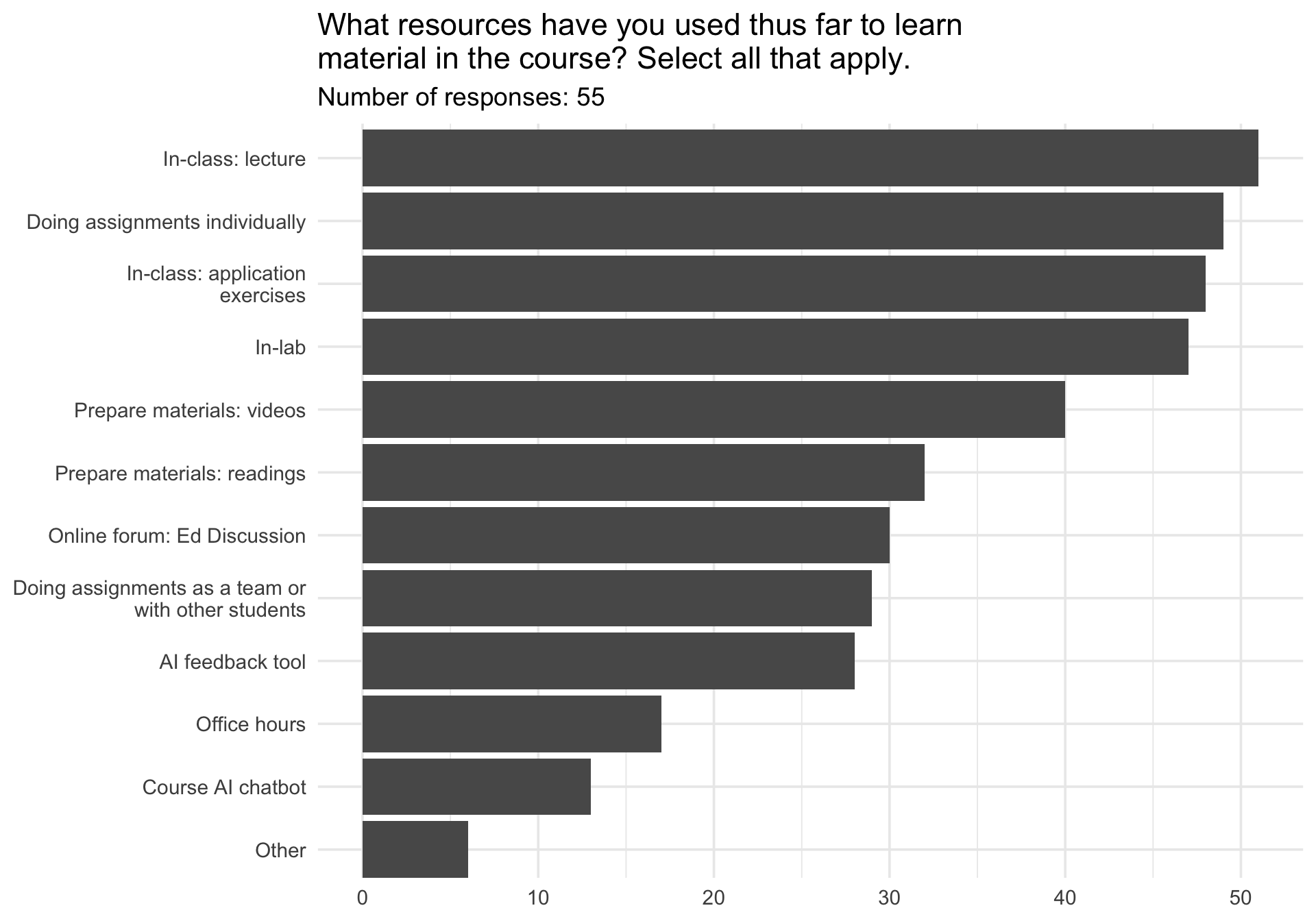
Midsemester survey results

Linear regression with a single predictor

Packages

library(tidyverse)
library(tidymodels)
library(fivethirtyeight)

Data prep

Rename Rotten Tomatoes columns as critics and audience
Rename the dataset as movie_scores

movie_scores <- fandango |>
  rename(
    critics = rottentomatoes,
    audience = rottentomatoes_user
  )

Data overview

movie_scores |>
  select(critics, audience)

# A tibble: 146 × 2
   critics audience
     <int>    <int>
 1      74       86
 2      85       80
 3      80       90
 4      18       84
 5      14       28
 6      63       62
 7      42       53
 8      86       64
 9      99       82
10      89       87
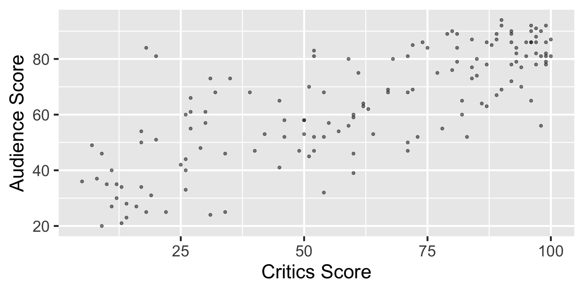
# ℹ 136 more rows

Data visualization

ggplot(movie_scores, aes(x = critics, y = audience)) +
  geom_point(alpha = 0.5) +
  labs(
    x = "Critics Score",
    y = "Audience Score"
  )

Regression model

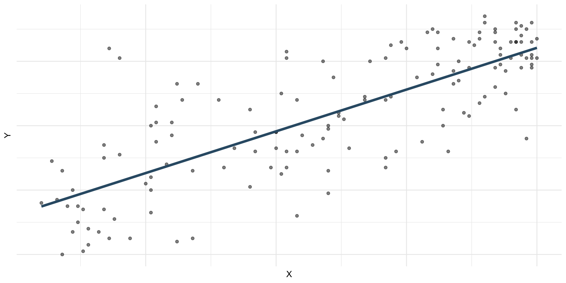
A regression model is a function that describes the relationship between the outcome, \(Y\), and the predictor, \(X\).

\[ \begin{aligned} Y &= \color{black}{\textbf{Model}} + \text{Error} \\[8pt] &= \color{black}{\mathbf{f(X)}} + \epsilon \\[8pt] &= \color{black}{\boldsymbol{\mu_{Y|X}}} + \epsilon \end{aligned} \]

Regression model

\[ \begin{aligned} Y &= \color{#325b74}{\textbf{Model}} + \text{Error} \\[8pt] &= \color{#325b74}{\mathbf{f(X)}} + \epsilon \\[8pt] &= \color{#325b74}{\boldsymbol{\mu_{Y|X}}} + \epsilon \end{aligned} \]

Simple linear regression

Use simple linear regression to model the relationship between a quantitative outcome (\(Y\)) and a single quantitative predictor (\(X\)): \[\Large{Y = \beta_0 + \beta_1 X + \epsilon}\]

\(\beta_1\): True slope of the relationship between \(X\) and \(Y\)
\(\beta_0\): True intercept of the relationship between \(X\) and \(Y\)
\(\epsilon\): Error (residual)

Simple linear regression

\[ \Large{\hat{Y} = b_0 + b_1 X} \]

\(b_1\): Estimated slope of the relationship between \(X\) and \(Y\)
\(b_0\): Estimated intercept of the relationship between \(X\) and \(Y\)
No error term!

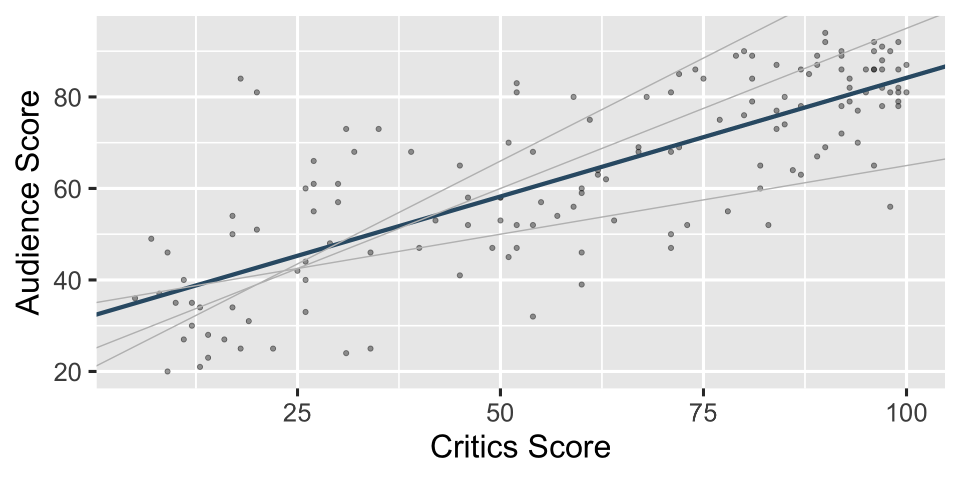
Choosing values for \(b_1\) and \(b_0\)

Residuals

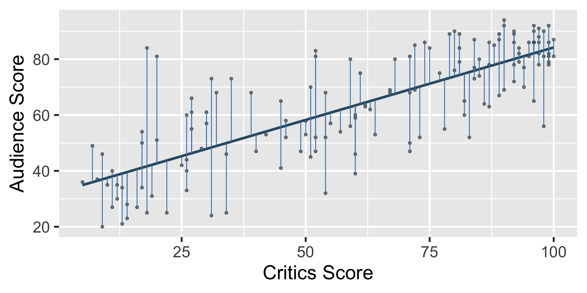
\[ \text{residual} = \text{observed} - \text{predicted} = y - \hat{y} \]

Least squares line

The residual for the \(i^{th}\) observation is

\[ e_i = \text{observed} - \text{predicted} = y_i - \hat{y}_i \]

The sum of squared residuals is

\[ e^2_1 + e^2_2 + \dots + e^2_n \]

The least squares line is the one that minimizes the sum of squared residuals

Least squares line

movies_fit <- linear_reg() |>
  fit(audience ~ critics, data = movie_scores)

tidy(movies_fit)

# A tibble: 2 × 5
  term        estimate std.error statistic  p.value
  <chr>          <dbl>     <dbl>     <dbl>    <dbl>
1 (Intercept)   32.3      2.34        13.8 4.03e-28
2 critics        0.519    0.0345      15.0 2.70e-31

Slope and intercept

Properties of least squares regression

The regression line goes through the center of mass point (the coordinates corresponding to average \(X\) and average \(Y\)): \(b_0 = \bar{Y} - b_1~\bar{X}\)
Slope has the same sign as the correlation coefficient: \(b_1 = r \frac{s_Y}{s_X}\)
Sum of the residuals is zero: \(\sum_{i = 1}^n \epsilon_i = 0\)
Residuals and \(X\) values are uncorrelated

Participate 📱💻

The slope of the model for predicting audience score from critics score is 0.519. Which of the following is the best interpretation of this value?

\[\widehat{\text{audience}} = 32.3 + 0.519 \times \text{critics}\]

For every one point increase in the critics score, the audience score goes up by 0.519 points, on average.
For every one point increase in the critics score, we expect the audience score to be higher by 0.519 points, on average.
For every one point increase in the critics score, the audience score goes up by 0.519 points.
For every one point increase in the audience score, the critics score goes up by 0.519 points, on average.

Scan the QR code or go to app.wooclap.com/sta199. Log in with your Duke NetID.

Participate 📱💻

The intercept of the model for predicting audience score from critics score is 32.3. Which of the following is the best interpretation of this value?

\[\widehat{\text{audience}} = 32.3 + 0.519 \times \text{critics}\]

For movies with a critics score of 0 points, we expect the audience score to be 32.3 points, on average.
For movies with an audience score of 0 points, we expect the critics score to be 32.3 points, on average.
For every one point increase in the critics score, the audience score goes up by 32.3 points.
For movies with an audience score of 0 points, we expect the critics score to be 0.519 points, on average.

Scan the QR code or go to app.wooclap.com/sta199. Log in with your Duke NetID.

Is the intercept meaningful?

✅ The intercept is meaningful in context of the data if

the predictor can feasibly take values equal to or near zero or
the predictor has values near zero in the observed data

. . .

🛑 Otherwise, it might not be meaningful!

Application exercise

ae-13-modeling-penguins

Go to your ae project in RStudio.
If you haven’t yet done so, make sure all of your changes up to this point are committed and pushed, i.e., there’s nothing left in your Git pane.
If you haven’t yet done so, click Pull to get today’s application exercise file: ae-13-modeling-penguins.qmd.
Work through the application exercise in class, and render, commit, and push your edits.

Recap

Calculate the predicted body weights of penguins on Biscoe, Dream, and Torgersen islands by hand.

\[ \widehat{body~mass} = 4716 - 1003 \times islandDream - 1010 \times islandTorgersen \]

. . .

Biscoe: \(\widehat{body~mass} = 4716 - 1003 \times 0 - 1010 \times 0 = 4716\)

. . .

Dream: \(\widehat{body~mass} = 4716 - 1003 \times 1 - 1010 \times 0 = 3713\)

. . .

Torgersen: \(\widehat{body~mass} = 4716 - 1003 \times 0 - 1010 \times 1 = 3706\)

Models with categorical predictors

When the categorical predictor has many levels, they’re encoded to dummy variables.
The first level of the categorical variable is the baseline level. In a model with one categorical predictor, the intercept is the predicted value of the outcome for the baseline level (x = 0).
Each slope coefficient describes the difference between the predicted value of the outcome for that level of the categorical variable compared to the baseline level.