Suggested answers can be found here, but resist the urge to peek before you go through it yourself.
Part 1 - General Social Survey
The General Social Survey is a high-quality survey which gathers data on American society and opinions, conducted since 1972. This data set is a sample of 500 entries from the GSS, spanning years 1973-2018, including demographic markers and some economic variables.1
gss
# A tibble: 500 × 11
    year   age sex    college   partyid hompop hours income class finrela weight
   <dbl> <dbl> <fct>  <fct>     <fct>    <dbl> <dbl> <ord>  <fct> <fct>    <dbl>
 1  2014    36 male   degree    ind          3    50 $2500… midd… below …  0.896
 2  1994    34 female no degree rep          4    31 $2000… work… below …  1.08
 3  1998    24 male   degree    ind          1    40 $2500… work… below …  0.550
 4  1996    42 male   no degree ind          4    40 $2500… work… above …  1.09
 5  1994    31 male   degree    rep          2    40 $2500… midd… above …  1.08
 6  1996    32 female no degree rep          4    53 $2500… midd… average  1.09
 7  1990    48 female no degree dem          2    32 $2500… work… below …  1.06
 8  2016    36 female degree    ind          1    20 $2500… midd… above …  0.478
 9  2000    30 female degree    rep          5    40 $2500… midd… average  1.10
10  1998    33 female no degree dem          2    40 $1500… work… far be…  0.550
# ℹ 490 more rows
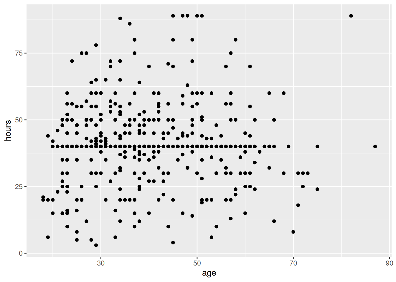
Suppose you want to estimate the correlation between hours (number of hours worked in week before survey, truncated at 89) and age (age at time of survey, truncated at 89).
Question 1
Which of the following is the best estimate of the correlation between hours and age?
-0.7
0
0.9
0.6
Question 2
Fill in the blank for the code below for computing the correlation between hours and age.
gss |>_____(r =cor(hours, age))
filter
mutate
summarize
group_by
Question 3
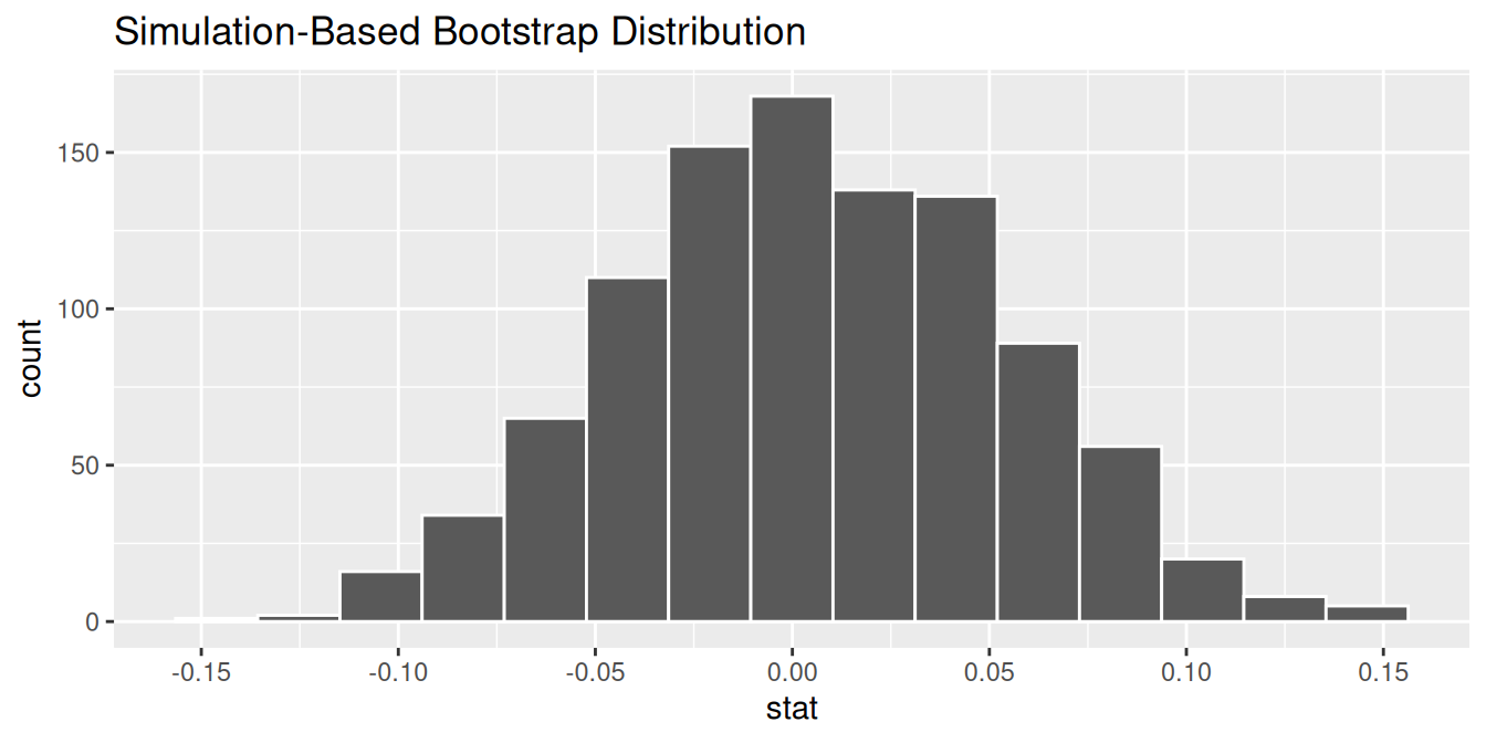
Fill in the blanks for the code below for simulating the bootstrap distribution of the correlation between hours and age using 10,000 bootstrap samples.
The bootstrap distribution from the previous question is visualized below. What is the approximate 95% confidence interval for the correlation between hours and age?
(-0.15, 0.15)
(-0.10, 0.10)
(-0.05, 0.05)
(0.05, 0.15)
Part 2 - Inference and modeling medley
Question 5
A survey based on a random sample of 2,045 American teenagers found that a 95% confidence interval for the mean number of texts sent per month was (1450, 1550). A valid interpretation of this interval is
95% of all teens who text send between 1450 and 1550 text messages per month.
If a new survey with the same sample size were to be taken, there is a 95% chance that the mean number of texts in the sample would be between 1450 and 1550.
We are 95% confident that the mean number of texts per month of all American teens is between 1450 and 1550.
We are 95% confident that, were we to repeat this survey, the mean number of texts per month of those taking part in the survey would be between 1450 and 1550.
Question 6
Which of the following is true about bootstrapping?
Bootstrap samples are drawn from the original sample with replacement.
Bootstrap samples are the same size (n) as our original sample.
The bootstrap uses the original sample to approximate the entire population.
All of the above.
Question 7
If the p-value is 0.06 and our discernibility level is 0.01, what do we do?
Accept the null.
Fail to reject the null.
Reject the null.
Eat the null.
Question 8
If the p-value is 0.0342 and our discernibility level is 0.05, what do we do?
Reject the null.
Accept the null.
Fail to reject the null.
Punch the null. In the face.
Question 9
In logistic regression, the response variable y is what type?
Numerical continuous.
Numerical discrete.
Categorical with two levels.
Categorical with three levels.
Question 10
A logistic regression model misclassifies an email from your grandmother as spam. That’s an example of a…
False positive.
False negative.
Question 11
What is sampling variability?
The variability of the outcome variable.
The variability of a statistic across different samples from the same population.
The difference between a treatment and control group.
The variability across different models.
Question 12
How much of a distribution is to the right of its 0.975 quantile?
0.975%
2.5%
50%
97.5%
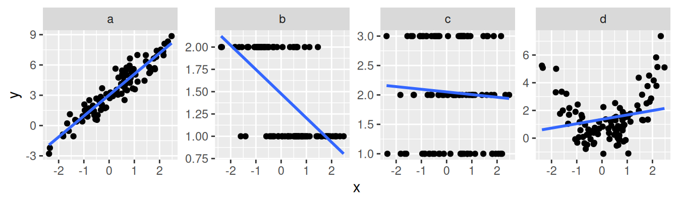
Question 13
In which case is a linear model most appropriate?
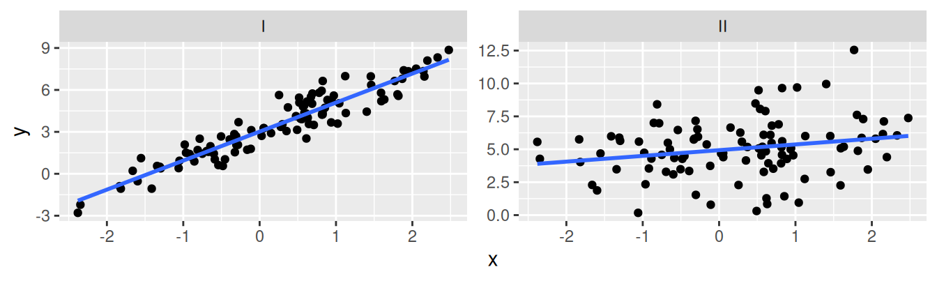
Question 14
Which of the following is true about the models below? Note that both models are fit to equally sized datasets (n = 100).
AUC of Model I > AUC of Model II
p-value of Model I > p-value of Model II
R-squared of Model I > R-squared of Model II
Log-odds of Model I > Log-odds of Model II
Question 15
Which is bigger?
A researcher is planning to conduct a test of two proportions. The null hypothesis is \(H_0: p_1 - p_2 = 0\). The researcher has found that in their data \(\hat{p}_1 - \hat{p}_2 = 0.2\).
I. p-value associated if \(H_A: p_1 - p_2 \ne 0\)
p-value associated if \(H_A: p_1 - p_2 > 0\)
I > II
I < II
I = II
Question 16
True or false. And, if false, explain your reasoning.
Increasing the number of bootstrap samples will decrease the width of the confidence interval.
Question 17
True or false. And, if false, explain your reasoning.
The bootstrap distribution of a sample proportion, \(\hat{p}\), will be centered at \(\hat{p}\).