# A tibble: 409 × 4
   percent_incr salary_type annual_salary performance_rating
          <dbl> <chr>               <dbl> <chr>
 1          1   Salaried               1  High
 2          1   Salaried               1  Successful
 3          1   Salaried               1  High
 4          1   Hourly             33987. Successful
 5         NA   Hourly             34798. High
 6         NA   Hourly             35360  <NA>
 7         NA   Hourly             37440  <NA>
 8          0   Hourly             37814. <NA>
 9          4   Hourly             41101. Top
10          1.2 Hourly             42328  <NA>
# ℹ 399 more rowsExam 1 review
Questions
Note
Suggested answers can be found here, but resist the urge to peek before you go through it yourself.
Blizzard salaries
In 2020, employees of Blizzard Entertainment circulated a spreadsheet to anonymously share salaries and recent pay increases amidst rising tension in the video game industry over wage disparities and executive compensation. (Source: Blizzard Workers Share Salaries in Revolt Over Pay)
The name of the data frame used for this analysis is blizzard_salary and the variables are:
percent_incr: Raise given in July 2020, as percent increase with values ranging from 1 (1% increase) to 21.5 (21.5% increase)salary_type: Type of salary, with levelsHourlyandSalariedannual_salary: Annual salary, in USD, with values ranging from $50,939 to $216,856.performance_rating: Most recent review performance rating, with levelsPoor,Successful,High, andTop. ThePoorlevel is the lowest rating and theToplevel is the highest rating.
The first ten rows of blizzard_salary are shown below:
Question 1
Which of the following is correct? Choose all that apply.
The
blizzard_salarydataset has 399 rows.The
blizzard_salarydataset has 4 columns.Each row represents a Blizzard Entertainment worker who filled out the spreadsheet.
The
percent_incrvariable is numerical and discrete.The
salary_typevariable is numerical.The
annual_salaryvariable is numerical.The
performance_ratingvariable is categorical and ordinal.
Question 2
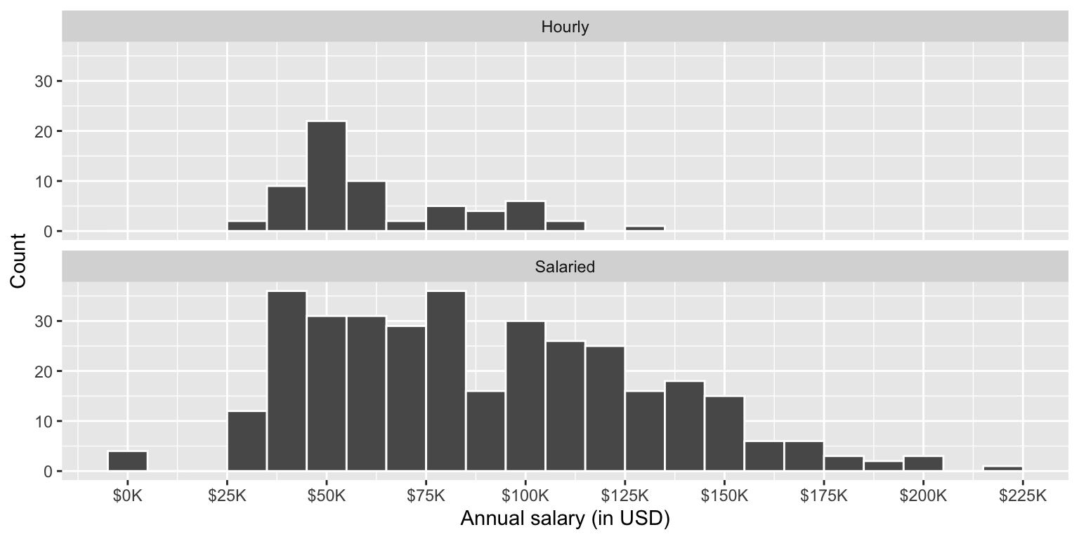
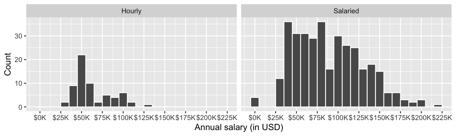
Figure 1 (a) and Figure 1 (b) show the distributions of annual salaries of hourly and salaried workers. The two figures show the same data, with the facets organized across rows and across columns. Which of the two figures is better for comparing the median annual salaries of hourly and salaried workers. Explain your reasoning.
Question 3
Suppose your teammate wrote the following code as part of their analysis of the data.
They then printed out the results shown below. Unfortunately one of the numbers got erased from the printout. It’s indicated with _____ below.
# A tibble: 2 × 3
  salary_type mean_annual_salary median_annual_salary
  <chr>                    <dbl>                <dbl>
1 Hourly                  63003.               54246.
2 Salaried                90183.               _____
Which of the following is the best estimate for that erased value?
30,000
50,000
80,000
100,000
Question 4
Which distribution of annual salaries has a higher standard deviation?
Hourly workers
Salaried workers
Roughly the same
Question 5
Which of the following alternate plots would also be useful for visualizing the distributions of annual salaries of hourly and salaried workers? Choose all that apply.
a. Box plots
b. Density plots
c. Pie charts
d. Waffle charts
e. Histograms
f. Scatterplots
Questions 6 and 7
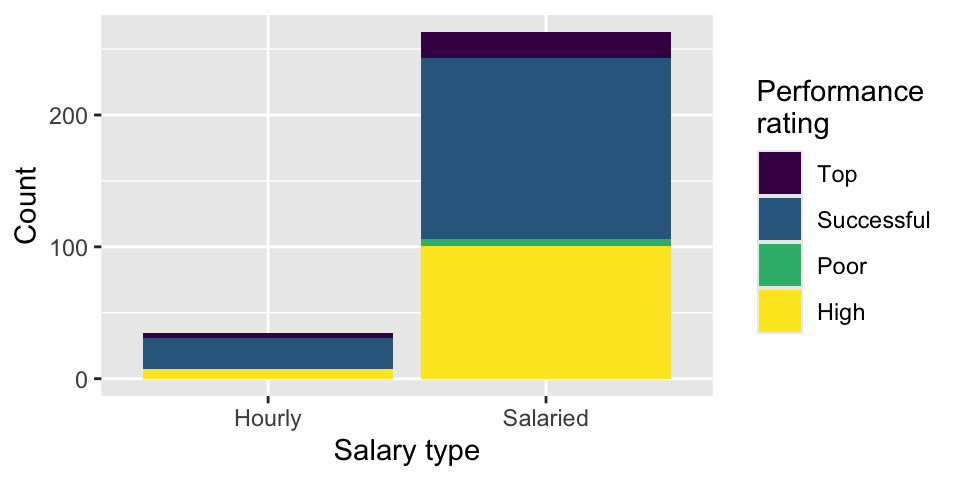
Suppose you made the bar plot shown in Figure 2 (a) to visualize the distribution of performance_rating and your teammate made the bar plot shown in Figure 2 (b).
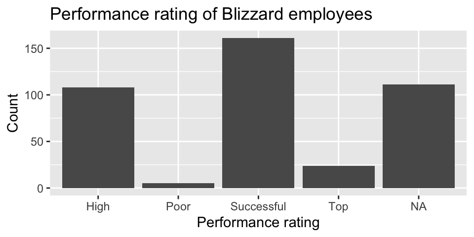
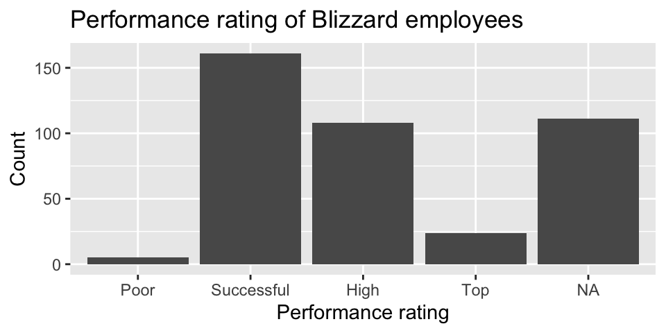
You made your bar plot without transforming the data in any way, while your friend did first transform the data with code like the following:
blizzard_salary <- blizzard_salary |>
  _(1)_(performance_rating = fct_relevel(performance_rating, _(2)_))
Question 6: What goes in the blank (1)?
arrange()mutate()summarize()
Question 7: What goes in the blank (2)?
"Poor", "Successful", "High", "Top""Successful", "High", "Top""Top", "High", "Successful", "Poor"Poor, Successful, High, Top
Questions 8 - 10
Finally, another teammate creates the following two plots.
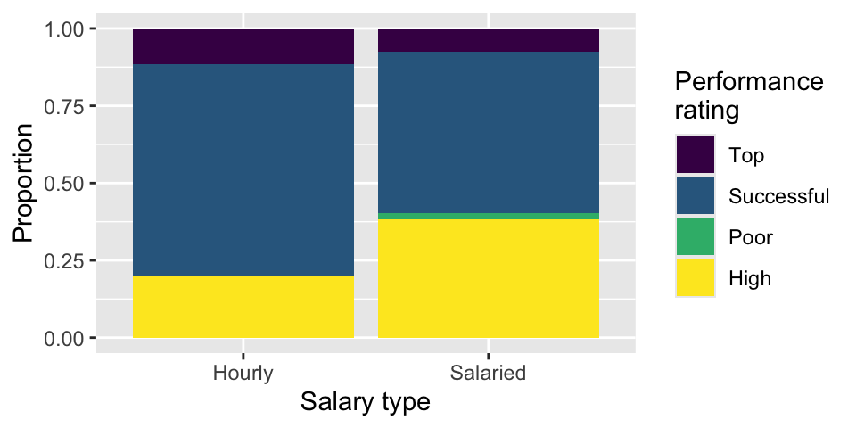
Question 8: Your teammate asks you for help deciding which one to use in the final report for visualizing the relationship between performance rating and salary type. In 1-3 sentences, can you help them make a decision, justify your choice, and write the narrative that should go with the plot?
Question 9: A friend with a keen eye points out that the number of observations in Figure 3 (a) seems lower than the total number of observations in blizzard_salary. What might be going on here? Explain your reasoning.
Question 10: Below are the proportions of performance ratings for hourly and salaried workers. Place these values in the corresponding segments in Figure 3 (b).
# A tibble: 4 × 3
  performance_rating Hourly Salaried
  <chr>               <dbl>    <dbl>
1 High                0.2     0.384
2 Successful          0.686   0.521
3 Top                 0.114   0.0760
4 Poor                0       0.0190
Questions 11 and 12
The table below shows the distribution of salary_type and performance_rating.
# A tibble: 2 × 6
  salary_type  Poor Successful  High   Top  `NA`
  <chr>       <int>      <int> <int> <int> <int>
1 Hourly         NA         24     7     4    28
2 Salaried        5        137   101    20    83
The pipeline below produces a data frame with a fewer number of rows than blizzard_salary.
blizzard_salary |>
  filter(salary_type _(1)_ "Hourly" _(2)_ performance_rating == "Poor") |>
  _(3)_(annual_salary)
# A tibble: 5 × 4
percent_incr salary_type annual_salary performance_rating
<dbl> <chr> <dbl> <chr>
1 0 Salaried 80000 Poor
2 3 Salaried 83000 Poor
3 0 Salaried 116000 Poor
4 0 Salaried 135219 Poor
5 0 Salaried 147500 Poor Question 11: Which of the following goes in blanks (1) and (2)?
| (1) | (2) | |
|---|---|---|
| a. | != |
| |
| b. | == |
& |
| c. | != |
& |
| d. | == |
| |
Question 12: Which function or functions go into blank (3)?
Question 13
You’re reviewing another team’s work and they made the following visualization:
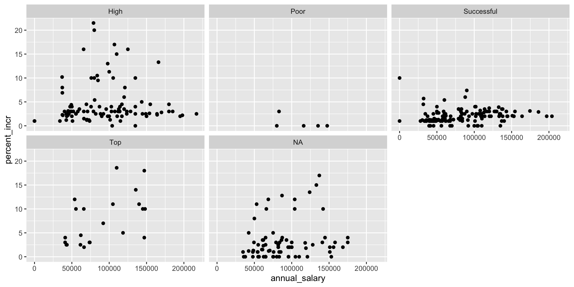
And they wrote the following interpretation for the relationship between annual salary and percent increase for Top performers:
The relationship is positive, having a higher salary results in a higher percent increase. There is one clear outlier.
Which of the following is/are the most accurate and helpful) peer review note for this interpretation. Choose all that apply.
The interpretation is complete and perfect, no changes needed!
The interpretation doesn’t mention the direction of the relationship.
The interpretation doesn’t mention the form of the relationship, which is linear.
The interpretation doesn’t mention the strength of the relationship, which is somewhat strong.
There isn’t a clear outlier in the plot. If any points stand out as potential outliers, more guidance should be given to the reader to identify them (e.g., salary and/or percent increase amount).
The interpretation is causal – we don’t know if the cause of the high percent increase is higher annual salary based on observational data. The causal direction might be the other way around, or there may be other factors contributing to the apparent relationship.
Question 14
Below is some code and its output.
```{r}
# label=plot blizzard

ggplot(blizzard_salary,aes(x=performance_rating,y=percent_incr))+geom_boxplot()
labs(x="Performance rating", y = "Percent increase")
```
Warning: Removed 39 rows containing non-finite outside the scale range
(`stat_boxplot()`).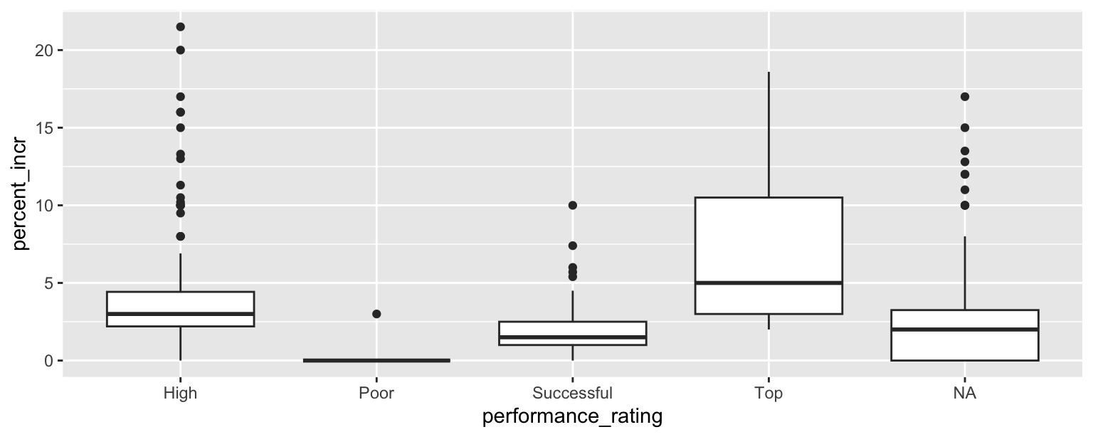
<ggplot2::labels> List of 2
 $ x: chr "Performance rating"
 $ y: chr "Percent increase"
Part 1: List at least 5 things that should be fixed or improved in the code.
Part 2: What is the cause of the warning and what does it mean?
Question 15
You’re working on a data analysis on salaries of Blizzard employees in a Quarto document in a project version controlled by Git. You create a plot and write up a paragraph describing any patterns in it. Then, your teammate says “render, commit, and push”.
Part 1: What do they mean by each of these three steps. In 1-2 sentences for each, explain in your own words what they mean.
- Render:
- Commit:
- Push:
Part 2: Your teammate is getting impatient and they interrupt you after you rendered and committed and say “I still can’t see your changes in our shared GitHub repo when I look at it in my web browser.” Which of the following answers is the most accurate?
I rendered my document, you should be seeing my changes on GitHub when you look at it in your web browser.
I committed my changes, you should be seeing my changes on GitHub when you look at it in your web browser.
I didn’t yet push my changes, it’s expected that you are not seeing them on GitHub when you look at it in your web browser. Wait until I push, and check again.
You need to pull to see my changes on GitHub in the web browser.
Penguins
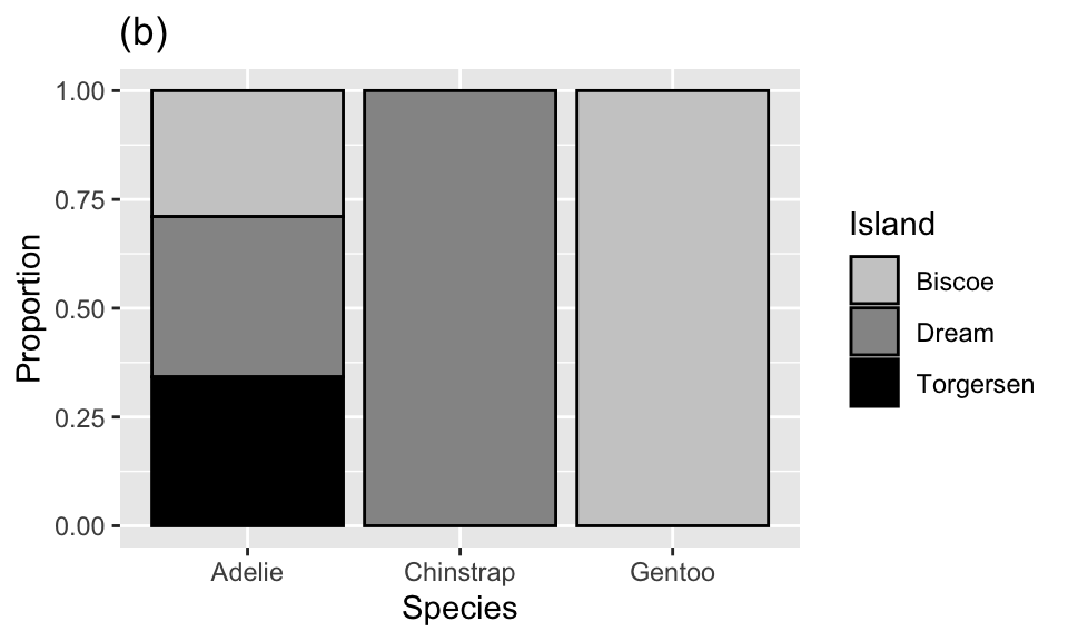
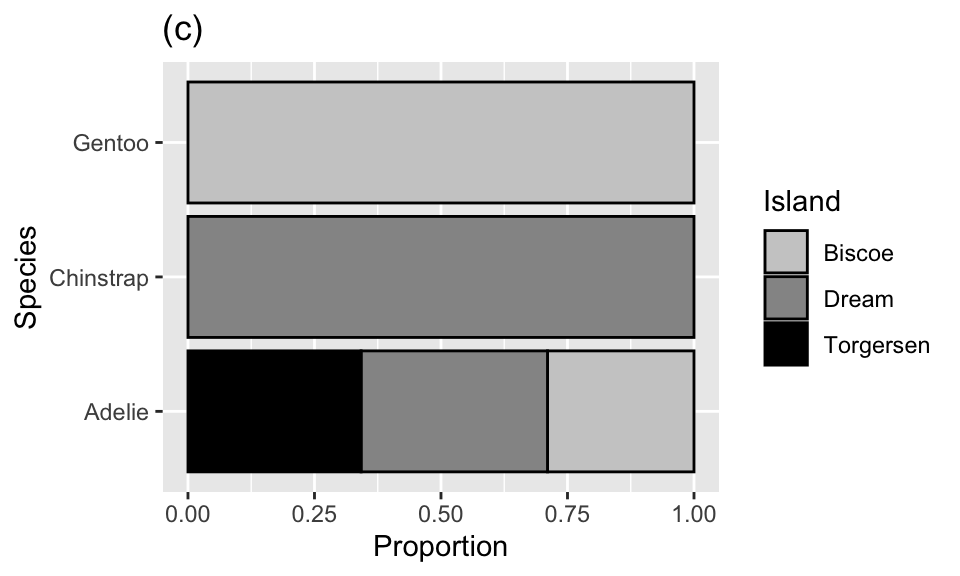
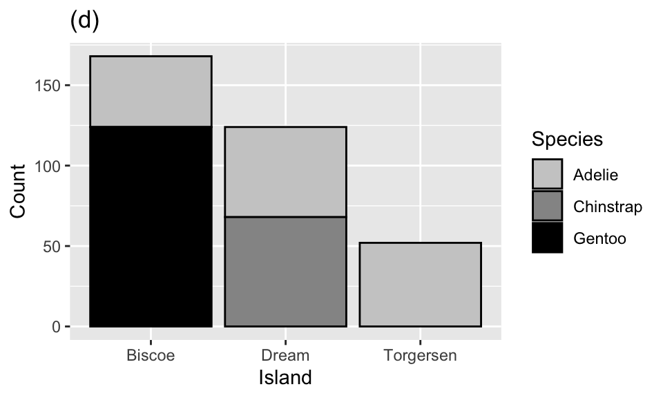
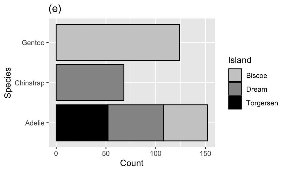
The penguins data set includes measurements for penguin species, including: flipper length, body mass, bill dimensions, and sex. The following table summarizes information on which species of penguins (Adelie, Gentoo, and Chinstrap) live on which islands (Biscoe, Dream, or Torgersen).
| Island | Adelie | Gentoo | Chinstrap | Total |
|---|---|---|---|---|
| Biscoe | 44 | 124 | 0 | 168 |
| Dream | 56 | 0 | 68 | 124 |
| Torgersen | 52 | 0 | 0 | 52 |
| Total | 152 | 124 | 68 | 344 |
Question 16
Which of the following plots is the result of the following code?
ggplot(penguins, aes(x = island, fill = species)) +
  geom_bar()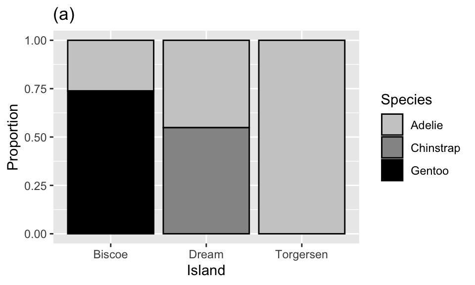
NYC Flights
The flights dataset includes characteristics of all flights departing from New York City airports (JFK, LGA, EWR) in 2013. Below is a peek at the first ten rows of the flights data.
# A tibble: 336,776 × 19
    year month   day arr_delay carrier dep_time sched_dep_time dep_delay
   <int> <int> <int>     <dbl> <chr>      <int>          <int>     <dbl>
 1  2013     1     1        11 UA           517            515         2
 2  2013     1     1        20 UA           533            529         4
 3  2013     1     1        33 AA           542            540         2
 4  2013     1     1       -18 B6           544            545        -1
 5  2013     1     1       -25 DL           554            600        -6
 6  2013     1     1        12 UA           554            558        -4
 7  2013     1     1        19 B6           555            600        -5
 8  2013     1     1       -14 EV           557            600        -3
 9  2013     1     1        -8 B6           557            600        -3
10  2013     1     1         8 AA           558            600        -2
# ℹ 336,766 more rows
# ℹ 11 more variables: arr_time <int>, sched_arr_time <int>, flight <int>,
#   tailnum <chr>, origin <chr>, dest <chr>, air_time <dbl>, distance <dbl>,
#   hour <dbl>, minute <dbl>, time_hour <dttm>
Question 17
Based on this output, which of the following must be true about the flights data frame? Select all that are true.
The
flightsdata frame is atibble.The
flightsdata frame has 10 rows.The
flightsdata frame has 8 columns.The
carriervariable in theflightsdata frame is a character variable.There are no missing data in the
flightsdata frame.
Question 18
Which of the following pipelines produce(s) the output shown below? Select all that apply.
# A tibble: 336,776 × 5
   arr_delay carrier  year month   day
       <dbl> <chr>   <int> <int> <int>
 1      1272 HA       2013     1     9
 2      1127 MQ       2013     6    15
 3      1109 MQ       2013     1    10
 4      1007 AA       2013     9    20
 5       989 MQ       2013     7    22
 6       931 DL       2013     4    10
 7       915 DL       2013     3    17
 8       895 DL       2013     7    22
 9       878 AA       2013    12     5
10       875 MQ       2013     5     3
# ℹ 336,766 more rows
a.
flights |>
  select(arr_delay, carrier, year, month, day) |>
  arrange(desc(arr_delay))
b.
flights |>
  select(arr_delay, carrier, year, month, day) |>
  arrange(arr_delay)
c.
flights |>
  select(arr_delay, carrier, year, month, day) |>
  arrange(year)
d.
flights |>
  arrange(desc(arr_delay)) |>
  select(arr_delay, carrier, year, month, day)
e.
flights |>
  arrange(desc(arr_delay)) |>
  select(day, month, year, arr_delay, carrier)
Countries and populations
We have a small dataset of six countries and their populations:
# A tibble: 6 × 2
  country       population
  <chr>              <dbl>
1 Curacao            150
2 Ecuador          18001
3 Iraq             44496.
4 New Zealand       5124.
5 Palau               18.0
6 United States   333288.
And another small dataset of five countries and the continent they’re in:
# A tibble: 5 × 3
  entity      code  continent
  <chr>       <chr> <chr>
1 Angola      AGO   Africa
2 Curacao     CUW   North America
3 Ecuador     ECU   South America
4 Iraq        IRQ   Asia
5 New Zealand NZL   Oceania
You join the two datasets with the following:
population |>
  left_join(continents, by = join_by(country == entity))
Question 19
How many rows will the resulting data frame have?
- 4
- 5
- 6
- 7
- 8
Question 20
What will be the columns of the resulting data frame?
country,populationcountry,population,code,continententity,code,continententity,population,code,continentcountry,entity,population,code,continent
Duke Forest houses
The duke_forest dataset includes information on prices and various other features (number of bedrooms, bathrooms, area, year built, type of cooling, type of heating, etc.) of houses in the Duke Forest neighborhood of Durham, NC.
Rows: 98
Columns: 13
$ address    <chr> "1 Learned Pl, Durham, NC 27705", "1616 Pinecrest Rd, Durha…
$ price      <dbl> 1520000, 1030000, 420000, 680000, 428500, 456000, 1270000, …
$ bed        <dbl> 3, 5, 2, 4, 4, 3, 5, 4, 4, 3, 4, 4, 3, 5, 4, 5, 3, 4, 4, 3,…
$ bath       <dbl> 4.0, 4.0, 3.0, 3.0, 3.0, 3.0, 5.0, 3.0, 5.0, 2.0, 3.0, 3.0,…
$ area       <dbl> 6040, 4475, 1745, 2091, 1772, 1950, 3909, 2841, 3924, 2173,…
$ type       <chr> "Single Family", "Single Family", "Single Family", "Single …
$ year_built <dbl> 1972, 1969, 1959, 1961, 2020, 2014, 1968, 1973, 1972, 1964,…
$ heating    <chr> "Other, Gas", "Forced air, Gas", "Forced air, Gas", "Heat p…
$ cooling    <fct> central, central, central, central, central, central, centr…
$ parking    <chr> "0 spaces", "Carport, Covered", "Garage - Attached, Covered…
$ lot        <dbl> 0.97, 1.38, 0.51, 0.84, 0.16, 0.45, 0.94, 0.79, 0.53, 0.73,…
$ hoa        <chr> NA, NA, NA, NA, NA, NA, NA, NA, NA, NA, NA, NA, NA, NA, NA,…
$ url        <chr> "https://www.zillow.com/homedetails/1-Learned-Pl-Durham-NC-…
The following summary table gives us some information about whether homes in this data set have garages and when they were built.
| Built earlier than 1950 | Built in 1950 or later | |
|---|---|---|
| Garage | 5 | 33 |
| No garage | 3 | 57 |
The pipeline below produces a data frame with a fewer number of rows than duke_forest.
duke_forest |>
  filter(parking == "Garage" _(1)_ year_built _(2)_ 1950) |>
  select(parking, year_built, price, area) |>
  _(3)_(price_per_sqfeet = price / area)
# A tibble: 5 × 5
parking year_built price area price_per_sqfeet
<chr> <dbl> <dbl> <dbl> <dbl>
1 Garage 1945 900000 2933 307.
2 Garage 1938 265000 1300 204.
3 Garage 1934 600000 2514 239.
4 Garage 1941 412500 1661 248.
5 Garage 1940 105000 1094 96.0Question 21
Which of the following goes in blanks (1) and (2)?
| (1) | (2) | |
|---|---|---|
| a. | & |
< |
| b. | | |
< |
| c. | & |
>= |
| d. | | |
>= |
| e. | & |
!= |
Question 22
Which function or functions go into blank (3)? Select all that apply.
arrange()mutate()summarize()slice()
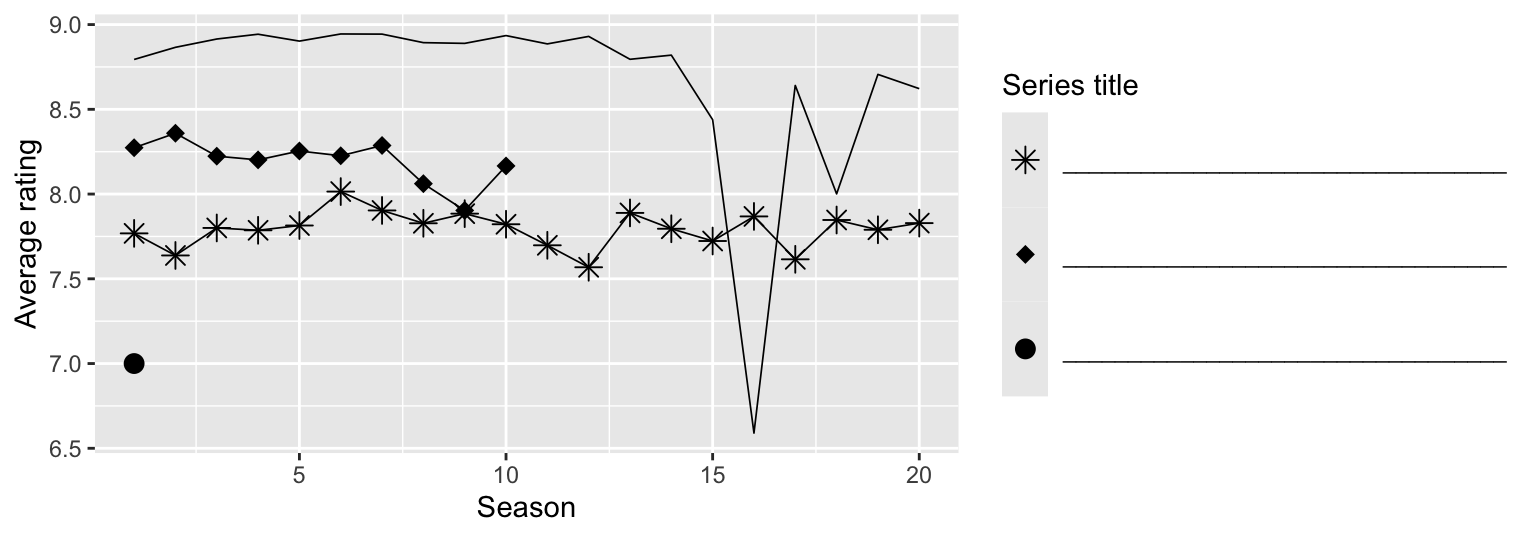
Law & Order
You’ve heard of the tidyverse, now let’s visit the Law & Order-verse. Doink doink!1
Law & Order is a police procedural and legal drama television series that has been running since the 1990s. The Law & Order franchise includes a number of series such as Law & Order, Law & Order: SVU, Law & Order: Criminal Intent, etc.
You will work with data on average ratings for each season of three series from the Law & Order-verse – a subset of the data from the previous questions. Below is a peek at the first ten rows of the Law & Order data.
The plot below shows the distributions of average ratings of various Law & Order series across seasons.
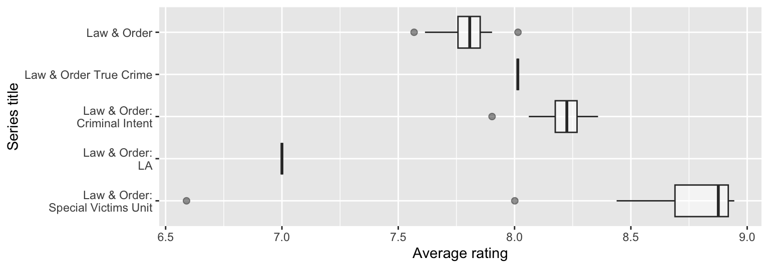
Question 23
Based on the information from the side-by-side box plots, fill in the legend of the plot below with Law & Order series titles.
Question 24
The following code calculates the standard deviations of average season ratings of the five Law & Order series. Unfortunately, the output is partially erased and replaced with blanks.
# A tibble: 5 × 3
  title                         mean_av_rating sd_av_rating
  <chr>                                  <dbl>        <dbl>
1 Law & Order                            _(1)_        0.106
2 Law & Order: Criminal Intent            8.20        0.129
4 Law & Order: SVU                        8.67        _(2)_
Based on the visualizations you’ve seen of these data so far, which of the following is true about the blanks in the output? Select all that are true.
The mean of average ratings (Blank 1) of Law & Order seasons is lower than the other two means.
The mean of average ratings (Blank 1) of Law & Order seasons is higher than the other two means.
The standard deviation of average ratings of Law & Order: SVU seasons (Blank 2) is lower than the other two standard deviations.
The standard deviation of average ratings of Law & Order: SVU seasons (Blank 2) is higher than the other two standard deviations.
The standard deviation of average ratings of Law & Order: SVU seasons (Blank 2) is between the other two standard deviations.
Romance and comedy
Finally, we focus on romance and comedy shows. We first filter the dataset for any shows that have romance or comedy as their genre (genre_1, genre_2, or genre_3) and then remove shows that have both of these genre labels. For the next two questions, we focus on these shows that we identify as either romance or comedy. We then calculate the mean of the average season ratings for each show, to obtain a single “mean average rating” value per show.
The plot below shows the distributions of mean average ratings of seasons of comedy and romance shows.
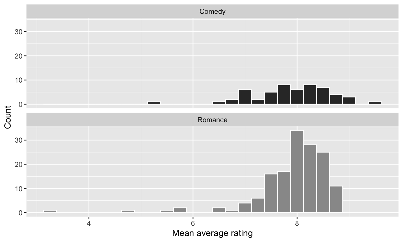
Question 25
Which of the following statements is true about these distributions? Select all that are true.
- Mean average ratings of romance shows are bimodal.
- Mean average ratings of comedy are unimodal.
- Mean average ratings of romance shows is left skewed.
- Mean average ratings of comedy shows is right skewed.
- There are more romance shows than comedy shows.
IMDB
The data for the next few questions come from the Internet Movie Database (IMDB). Specifically, the data are a random sample of movies released between 1980 and 2020.
The name of the data frame used for this analysis is movies, and it contains the variables shown in Table 1.
movies
| Variable | Description |
|---|---|
name |
name of the movie |
rating |
rating of the movie (R, PG, etc.) |
genre |
main genre of the movie. |
runtime |
duration of the movie |
year |
year of release |
release_date |
release date (YYYY-MM-DD) |
release_country |
release country |
score |
IMDB user rating |
votes |
number of user votes |
director |
the director |
writer |
writer of the movie |
star |
main actor/actress |
country |
country of origin |
budget |
the budget of a movie (some movies don’t have this, so it appears as 0) |
gross |
revenue of the movie |
company |
the production company |
The first thirty rows of the movies data frame are shown in Table 2, with variable types suppressed (since we’ll ask about them later).
First 30 rows of movies, with variable types suppressed.
# A tibble: 500 × 16
   name           score runtime genre     rating    release_country release_date
 1 Blue City        4.4 83 mins Action    R         United States   1986-05-02
 2 Winter Sleep     8.1 196     Drama     Not Rated Turkey          2014-06-12
 3 Rang De Basan…   8.1 167     Comedy    Not Rated United States   2006-01-26
 4 Pokémon Detec…   6.6 104     Action    PG        United States   2019-05-10
 5 A Bad Moms Ch…   5.6 104     Comedy    R         United States   2017-11-01
 6 Replicas         5.5 107     Drama     PG-13     United States   2019-01-11
 7 Windy City       5.8 103     Drama     R         Uruguay         1986-01-01
 8 War for the P…   7.4 140     Action    PG-13     United States   2017-07-14
 9 Tales from th…   6.4 98      Crime     R         United States   1995-05-24
10 Fire with Fire   6.5 103     Drama     PG-13     United States   1986-05-09
11 Raising Helen    6   119     Comedy    PG-13     United States   2004-05-28
12 Feeling Minne…   5.4 99      Comedy    R         United States   1996-09-13
13 The Babe         5.9 115     Biography PG        United States   1992-04-17
14 The Real Blon…   6   105     Comedy    R         United States   1998-02-27
15 To vlemma tou…   7.6 176     Drama     Not Rated United States   1997-11-01
16 Going the Dis…   6.3 102     Comedy    R         United States   2010-09-03
17 Jung on zo       6.8 103     Action    R         Hong Kong       1993-06-24
18 Rita, Sue and…   6.5 93      Comedy    R         United Kingdom  1987-05-29
19 Phone Booth      7   81      Crime     R         United States   2003-04-04
20 Happy Death D…   6.6 96      Comedy    PG-13     United States   2017-10-13
21 Barely Legal     4.7 90      Comedy    R         Thailand        2006-05-25
22 Three Kings      7.1 114     Action    R         United States   1999-10-01
23 Menace II Soc…   7.5 97      Crime     R         United States   1993-05-26
24 Four Rooms       6.8 98      Comedy    R         United States   1995-12-25
25 Quartet          6.8 98      Comedy    PG-13     United States   2013-03-01
26 Tape             7.2 86      Drama     R         Denmark         2002-07-12
27 Marked for De…   6   93      Action    R         United States   1990-10-05
28 Congo            5.2 109     Action    PG-13     United States   1995-06-09
29 Stop-Loss        6.4 112     Drama     R         United States   2008-03-28
30 Con Air          6.9 115     Action    R         United States   1997-06-06
      budget     gross  votes  year director         writer        star

 1  10000000   6947787   1100  1986 Michelle Manning Ross Macdona… Judd Nelson
 2        NA   4018705  48000  2014 Nuri Bilge Ceyl… Ebru Ceylan   Haluk Bilgin…
 3        NA  10800778 115000  2006 Rakeysh Ompraka… Renzil D'Sil… Aamir Khan
 4 150000000 433921300 146000  2019 Rob Letterman    Dan Hernandez Ryan Reynolds
 5  28000000 130560428  46000  2017 Jon Lucas        Jon Lucas     Mila Kunis
 6  30000000   9330075  34000  2018 Jeffrey Nachman… Chad St. John Keanu Reeves
 7        NA    343890    262  1984 Armyan Bernstein Armyan Berns… John Shea
 8 150000000 490719763 235000  2017 Matt Reeves      Mark Bomback  Andy Serkis
 9   6000000  11837928   7400  1995 Rusty Cundieff   Rusty Cundie… Clarence Wil…
10        NA   4636169   1500  1986 Duncan Gibbins   Bill Phillips Craig Sheffer
11  50000000  49718611  36000  2004 Garry Marshall   Patrick J. C… Kate Hudson
12        NA   3124440  11000  1996 Steven Baigelman Steven Baige… Keanu Reeves
13        NA  19930973   9300  1992 Arthur Hiller    John Fusco    John Goodman
14        NA     83488   3900  1997 Tom DiCillo      Tom DiCillo   Matthew Modi…
15        NA        NA   6400  1995 Theodoros Angel… Theodoros An… Harvey Keitel
16  32000000  42059111  57000  2010 Nanette Burstein Geoff LaTuli… Drew Barrymo…
17        NA   3741869   6100  1993 Kirk Wong        Tin Nam Chun  Jackie Chan
18        NA    124167   3600  1987 Alan Clarke      Andrea Dunbar Siobhan Finn…
19  13000000  97837138 255000  2002 Joel Schumacher  Larry Cohen   Colin Farrell
20   4800000 125479266 124000  2017 Christopher Lan… Scott Lobdell Jessica Rothe
21        NA     83439   5900  2003 David Mickey Ev… David H. Ste… Erik von Det…
22  75000000 107752036 163000  1999 David O. Russell John Ridley   George Cloon…
23   3500000  27912072  54000  1993 Albert Hughes    Allen Hughes  Tyrin Turner
24   4000000   4257354 100000  1995 Directors        Allison Ande… Tim Roth
25  11000000  59520298  19000  2012 Dustin Hoffman   Ronald Harwo… Maggie Smith
26    100000    515900  19000  2001 Richard Linklat… Stephen Belb… Ethan Hawke
27  12000000  57968936  21000  1990 Dwight H. Little Michael Grais Steven Seagal
28  50000000 152022101  43000  1995 Frank Marshall   Michael Cric… Laura Linney
29  25000000  11212953  20000  2008 Kimberly Peirce  Mark Richard  Ryan Phillip…
30  75000000 224012234 282000  1997 Simon West       Scott Rosenb… Nicolas Cage
# ℹ 470 more rows
# ℹ 2 more variables: company, country
Question 26
The name and runtime variables are shown below, with the variable types suppressed.
# A tibble: 500 × 2
  name                      runtime
1 Blue City                 83 mins
2 Winter Sleep              196
3 Rang De Basanti           167
4 Pokémon Detective Pikachu 104
5 A Bad Moms Christmas      104
6 Replicas                  107
# ℹ 494 more rows
What is the type of the runtime variable?
Character
Double
Factor
Integer
Logical
Question 27
The code below summarizes the data in a certain way.
movies |>
  summarize(sum(release_country == "United States"))
# A tibble: 1 × 1
`sum(release_country == "United States")`
<int>
1 435Which of the following is TRUE about the code and its result? Select all that are true.
Evaluates whether each
release_countryis equal to"United States"or not, which results in a logical variable.Filters out rows where
release_countryis not equal to"United States"and counts the remaining rows.Sums the logical values, where each
TRUEis considered a 1 and eachFALSEis considered a 0.Results in a character vector.
The result shows there are 435 movies released in the United States.
Question 28
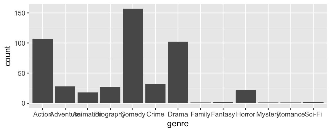
Suppose you want a visualization that shows the number of movies in the sample in each genre. Your first attempt is as follows.
A friend of yours says that the visualization is difficult to read and they suggest using the following visualization instead.
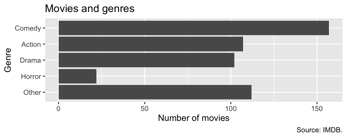
Which of the following modifications would your friend have made to your code to create their version? Select all that apply.
Combine movies in genres other than Comedy, Drama, Action, and Horror into a new level called
"Other".Reorder the levels in descending order of numbers of observations, except for the
"Other"level.Map
genreto theyaesthetic.Add a title, x and y-axis labels, and a caption.
Filter out all moves in genres other than Comedy, Drama, Action, and Horror before plotting.
Question 29
Which of the following is TRUE about the code and its result? Select all that are true.
movies |>
  count(rating, genre) |>
  pivot_wider(names_from = genre, values_from = n, values_fill = 0)
# A tibble: 6 × 6
rating Other Drama Action Comedy Horror
<fct> <int> <int> <int> <int> <int>
1 G 5 1 1 1 0
2 PG 38 13 10 18 0
3 PG-13 19 25 35 35 0
4 R 45 50 57 96 21
5 NC-17 1 2 0 1 0
6 Not Rated 4 11 4 6 1The code counts how many movies are in each rating and genre combination.
The code sorts the results in descending order.
Each row of the output is a movie.
The output shows that there are six distinct ratings in the dataset.
The code reduces the number of variables and observations in the
moviesdata frame to six.
Bonus
Pick a concept we introduced in class so far that you’ve been struggling with and explain it in your own words.
Footnotes
“Doink doink” is the scene and episode introductory sound on the Law & Order series. If you’ve never heard it, you’re not at any disadvantage for the exam. If you’ve ever heard it, good luck getting it out of your head!↩︎