AE 15: Houses in Duke Forest

Packages

We will use tidyverse and tidymodels for data exploration and modeling, respectively, and the openintro package for the data, and the knitr package for formatting tables.

library(tidyverse)
library(tidymodels)
library(openintro)
library(knitr)

Data

The data are on houses that were sold in the Duke Forest neighborhood of Durham, NC around November 2020. It was originally scraped from Zillow, and can be found in the duke_forest data set in the openintro R package.

glimpse(duke_forest)

Rows: 98
Columns: 13
$ address    <chr> "1 Learned Pl, Durham, NC 27705", "1616 Pinecrest Rd, Durha…
$ price      <dbl> 1520000, 1030000, 420000, 680000, 428500, 456000, 1270000, …
$ bed        <dbl> 3, 5, 2, 4, 4, 3, 5, 4, 4, 3, 4, 4, 3, 5, 4, 5, 3, 4, 4, 3,…
$ bath       <dbl> 4.0, 4.0, 3.0, 3.0, 3.0, 3.0, 5.0, 3.0, 5.0, 2.0, 3.0, 3.0,…
$ area       <dbl> 6040, 4475, 1745, 2091, 1772, 1950, 3909, 2841, 3924, 2173,…
$ type       <chr> "Single Family", "Single Family", "Single Family", "Single …
$ year_built <dbl> 1972, 1969, 1959, 1961, 2020, 2014, 1968, 1973, 1972, 1964,…
$ heating    <chr> "Other, Gas", "Forced air, Gas", "Forced air, Gas", "Heat p…
$ cooling    <fct> central, central, central, central, central, central, centr…
$ parking    <chr> "0 spaces", "Carport, Covered", "Garage - Attached, Covered…
$ lot        <dbl> 0.97, 1.38, 0.51, 0.84, 0.16, 0.45, 0.94, 0.79, 0.53, 0.73,…
$ hoa        <chr> NA, NA, NA, NA, NA, NA, NA, NA, NA, NA, NA, NA, NA, NA, NA,…
$ url        <chr> "https://www.zillow.com/homedetails/1-Learned-Pl-Durham-NC-…

Model

df_fit <- linear_reg() |>
  set_engine("lm") |>
  fit(price ~ area, data = duke_forest)

tidy(df_fit) |>
  kable(digits = 2)

term	estimate	std.error	statistic	p.value
(Intercept)	116652.33	53302.46	2.19	0.03
area	159.48	18.17	8.78	0.00

Bootstrap confidence interval

1. Calculate the observed fit (slope)

observed_fit <- duke_forest |>
  specify(price ~ area) |>
  fit()

observed_fit

# A tibble: 2 × 2
  term      estimate
  <chr>        <dbl>
1 intercept  116652.
2 area          159.

2. Take n bootstrap samples and fit models to each one.

Fill in the code, then set eval: true .

n = 100
set.seed(20251125)

boot_fits <- duke_forest |>
  specify(price ~ area) |>
  generate(reps = n, type = "bootstrap") |>
  fit()

boot_fits

# A tibble: 200 × 3
# Groups:   replicate [100]
   replicate term      estimate
       <int> <chr>        <dbl>
 1         1 intercept 340808. 
 2         1 area          73.4
 3         2 intercept  79713. 
 4         2 area         175. 
 5         3 intercept  85114. 
 6         3 area         183. 
 7         4 intercept 144051. 
 8         4 area         142. 
 9         5 intercept -55286. 
10         5 area         227. 
# ℹ 190 more rows

Why do we set a seed before taking the bootstrap samples?
Make a histogram of the bootstrap samples to visualize the bootstrap distribution.

boot_fits |>
  filter(term == "area") |>
  ggplot(aes(x = estimate)) +
  geom_histogram()

`stat_bin()` using `bins = 30`. Pick better value `binwidth`.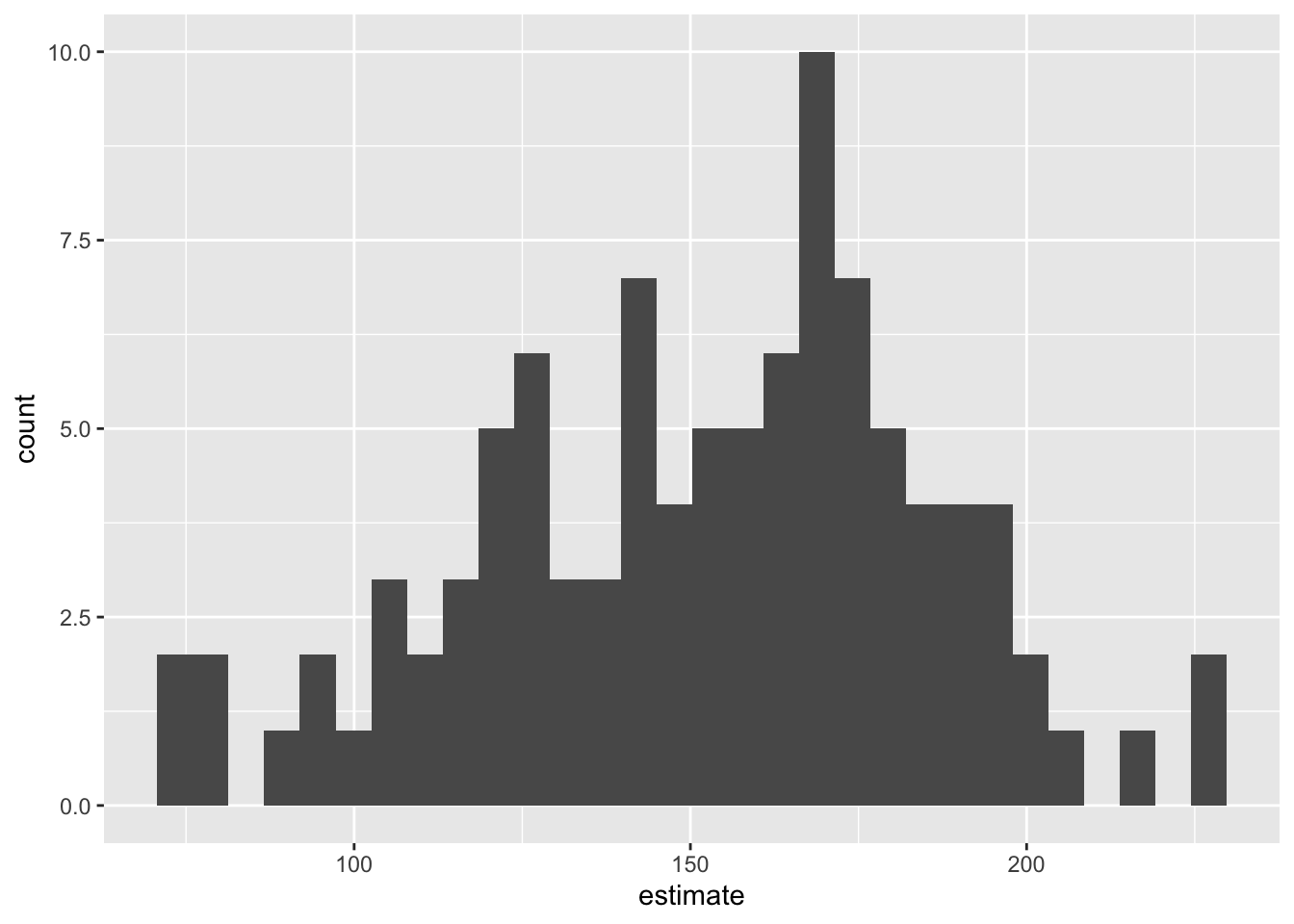

3. Compute the 95% confidence interval as the middle 95% of the bootstrap distribution

Fill in the code, then set eval: true .

get_confidence_interval(
  boot_fits,
  point_estimate = observed_fit,
  level = 0.95,
  type = "percentile"
)

# A tibble: 2 × 3
  term      lower_ci upper_ci
  <chr>        <dbl>    <dbl>
1 area          78.3     212.
2 intercept -18861.   297587.

Changing confidence level

Modify the code from Step 3 to create a 90% confidence interval.

get_confidence_interval(
  boot_fits,
  point_estimate = observed_fit,
  level = 0.90,
  type = "percentile"
)

# A tibble: 2 × 3
  term      lower_ci upper_ci
  <chr>        <dbl>    <dbl>
1 area          94.9     198.
2 intercept  21288.   289304.

Modify the code from Step 3 to create a 99% confidence interval.

get_confidence_interval(
  boot_fits,
  point_estimate = observed_fit,
  level = 0.99,
  type = "percentile"
)

# A tibble: 2 × 3
  term      lower_ci upper_ci
  <chr>        <dbl>    <dbl>
1 area          73.9     227.
2 intercept -59585.   330014.

Which confidence level produces the most accurate confidence interval (90%, 95%, 99%)? Explain
Which confidence level produces the most precise confidence interval (90%, 95%, 99%)? Explain
If we want to be very certain that we capture the population parameter, should we use a wider or a narrower interval? What drawbacks are associated with using a wider interval?