AE 04: Gerrymandering + data exploration II

Getting started

Packages

We’ll use the tidyverse package for this analysis.

library(tidyverse)
library(usdata)
library(ggbeeswarm)
library(ggthemes)
library(scales)

Data

The data are availale in the usdata package.

glimpse(gerrymander)

Rows: 435
Columns: 12
$ district   <chr> "AK-AL", "AL-01", "AL-02", "AL-03", "AL-04", "AL-05", "AL-0…
$ last_name  <chr> "Young", "Byrne", "Roby", "Rogers", "Aderholt", "Brooks", "…
$ first_name <chr> "Don", "Bradley", "Martha", "Mike D.", "Rob", "Mo", "Gary",…
$ party16    <chr> "R", "R", "R", "R", "R", "R", "R", "D", "R", "R", "R", "R",…
$ clinton16  <dbl> 37.6, 34.1, 33.0, 32.3, 17.4, 31.3, 26.1, 69.8, 30.2, 41.7,…
$ trump16    <dbl> 52.8, 63.5, 64.9, 65.3, 80.4, 64.7, 70.8, 28.6, 65.0, 52.4,…
$ dem16      <dbl> 0, 0, 0, 0, 0, 0, 0, 1, 0, 0, 0, 0, 1, 0, 1, 0, 0, 0, 1, 0,…
$ state      <chr> "AK", "AL", "AL", "AL", "AL", "AL", "AL", "AL", "AR", "AR",…
$ party18    <chr> "R", "R", "R", "R", "R", "R", "R", "D", "R", "R", "R", "R",…
$ dem18      <dbl> 0, 0, 0, 0, 0, 0, 0, 1, 0, 0, 0, 0, 1, 1, 1, 0, 0, 0, 1, 0,…
$ flip18     <dbl> 0, 0, 0, 0, 0, 0, 0, 0, 0, 0, 0, 0, 0, 1, 0, 0, 0, 0, 0, 0,…
$ gerry      <fct> mid, high, high, high, high, high, high, high, mid, mid, mi…

Congressional districts per state

Which state has the most congressional districts? How many congressional districts are there in this state?

gerrymander |>
  count(state, sort = TRUE)

# A tibble: 50 × 2
   state     n
   <chr> <int>
 1 CA       53
 2 TX       36
 3 FL       27
 4 NY       27
 5 IL       18
 6 PA       18
 7 OH       16
 8 GA       14
 9 MI       14
10 NC       13
# ℹ 40 more rows

Gerrymandering and flipping

Is a Congressional District more likely to be flipped to a Democratic seat if it has high prevalence of gerrymandering or low prevalence of gerrymandering? Support your answer with a visualization and summary statistics.

gerrymander |>
  mutate(flip18 = as.factor(flip18)) |>
  ggplot(aes(y = gerry, fill = flip18)) +
  geom_bar(position = "fill")

gerrymander |>
  count(gerry, dem18) |>
  group_by(gerry) |>
  mutate(p = n / sum(n))

# A tibble: 6 × 4
# Groups:   gerry [3]
  gerry dem18     n     p
  <fct> <dbl> <int> <dbl>
1 low       0    25 0.403
2 low       1    37 0.597
3 mid       0   131 0.485
4 mid       1   139 0.515
5 high      0    52 0.505
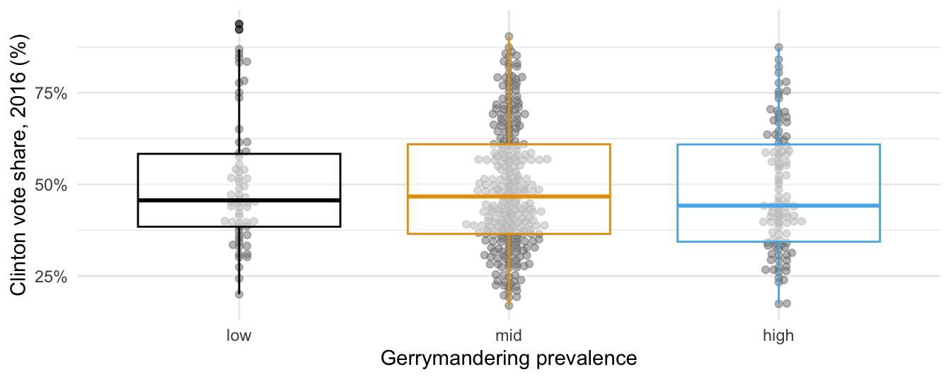
6 high      1    51 0.495

Aesthetic mappings

Recreate the following visualization, and then improve it.

ggplot(gerrymander, aes(x = gerry, y = clinton16)) +
  geom_beeswarm(color = "gray50", alpha = 0.5) +
  geom_boxplot(
    aes(color = gerry), 
    alpha = 0.5, 
    show.legend = FALSE
  ) +
  scale_color_colorblind() +
  scale_y_continuous(labels = label_percent(scale = 1)) +
  theme_minimal() +
  labs(
    x = "Gerrymandering prevalence",
    y = "Clinton vote share, 2016 (%)",
  )